Guided Grad-CAM for White Box Explainability of Image Classifiers

Convolution Neural Network expanded its task from Image classification to Image captioning. With the expansion of this task, the architecture of CNN has been evolving into a more complex structure. With the increase in complexity, interpretability has been a major challenge. Because of these interpretability issues, should we trust CNN models blindly? If not, have you ever wondered how the CNN model predicts? Or why it is predicting some class and not the other class?

In this article, we will be covering such questions by going through one of the Explainability techniques of the CNN model i.e. Guided GradCAM.

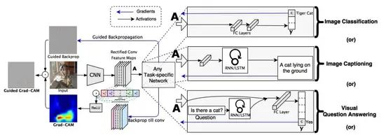
Guided GradCAM is a combination of two techniques i.e. Guided Backpropagation and GradCAM (Figure 1). Guided GradCAM will be applied to the pre-trained VGG16 model. Before moving forward with the Guided GradCAM technique, we will go through GradCAM and Guided Backpropagation techniques individually.

GradCAM (Gradient weighted Class Activation Map)

GradCAM is an Explainability technique where it produces the heat map, which indicates exactly where the model is focusing on the image. For this GradCAM needs to know the architecture of the model which makes it a white-box explainability testing and it provides more accurate results than black-box explainability testing.

VGG16 model is imported and an extra model is created, where it takes input as the original Image and its output will be the resultant of the last convolutional layer(i.e. "block5_conv3") of the VGG16 model.  The output of the last layer of convolution (14 x 14 x 512) is used mainly because it contains very important spatial information which is then Flattened and passed to the dense layer for prediction.

import numpy as np
import matplotlib.pyplot as plt
import tensorflow as tf
from tensorflow.keras.preprocessing.image import load_img
from tensorflow.keras.applications.vgg16 import VGG16,preprocess_input, decode_predictions

model = VGG16()
last_conv_layer = model.get_layer("block5_conv3")
last_conv_layer_model = tf.keras.Model(model.inputs, last_conv_layer.output)

classifier_input = tf.keras.Input(shape=last_conv_layer.output.shape[1:])
x = classifier_input
for layer_name in ["block5_pool","flatten","fc1","fc2", "predictions"]:
    x = model.get_layer(layer_name)(x)
classifier_model = tf.keras.Model(classifier_input, x)

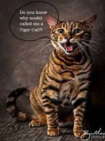
Image of Tiger Cat (Figure 2) will be used to understand explainability techniques

Mean of the partial derivative of VGG16’s output w.r.t each activation map is calculated

The above weight gives the weightage of each activation map for predicting the output. The ReLu of a weighted combination of activation maps will give a heat map that contains features that are positively influenced by a particular class.

Resultant of the above equation for the input image as a "Tiger cat"(Figure 2) is shown below in Figure 3.

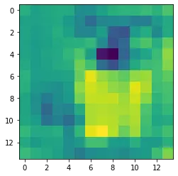
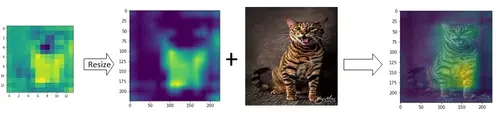
The above image is of size 14 x 14. which is actually resized to 224 x 224 and overlapped on the original image. The final image contains a heat map that indicates exactly where the model is focusing on the original image.

The above heat Map quite explains why the model predicted the image as a cat. We can understand from the above heat map that the model is mainly focusing on mostly the Body part and some of the face parts of the cat. But we are still unsure why the model predicted the image as specifically a “Tiger cat”?! Here comes the Guided Backpropagation to rescue

with tf.GradientTape() as tape:
    inputs = preprocess_input(image[np.newaxis, ...])
    last_conv_layer_output = last_conv_layer_model(inputs)
    tape.watch(last_conv_layer_output)
    preds = classifier_model(last_conv_layer_output)
    top_pred_index = tf.argmax(preds[0])
    top_class_channel = preds[:, top_pred_index]
grads = tape.gradient(top_class_channel, last_conv_layer_output) #Gradients of prediction and activation map of final convolution layer

pooled_grads = tf.reduce_mean(grads, axis=(0, 1, 2)) #mean of gradients

last_conv_layer_output = last_conv_layer_output.numpy()[0]
pooled_grads = pooled_grads.numpy()

for i in range(pooled_grads.shape[-1]):
    last_conv_layer_output[:, :, i] *= pooled_grads[i]  #weighted combination of activation map
    
gradcam = np.mean(last_conv_layer_output, axis=-1) 
gradcam = np.clip(gradcam, 0, np.max(gradcam)) / np.max(gradcam) #applying relu
gradcam = cv2.resize(gradcam, (224, 224))   #resizing

Guided Backpropagation

During the forward pass, we have many ReLu activations which clip the negative values to zero. Similarly during Backpropagation, we clip negative gradients to zero. This helps in neglecting all the negative influences (gradients) and focusing only on positive influences (gradients).

Guided backpropagation is achieved by a custom gradient function i.e. @tf.custom_gradient

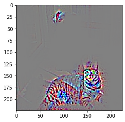
Element wise product of Guided Backpropagation and GradCAM will lead to Guided GradCAM which is shown in Figure 5

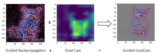
From the above Image, it is observed that, unlike GradCAM, Guided GradCAM highlights fine-grained pixel-level details. From Figure 5 it is observed that the VGG16 model is focusing on the stripes of the cat which is the reason why it predicted “Tiger cat”! Other than stripes, the model also focused on the face, ears, eyes, etc. which means the model has learned important features to determine this class.

What makes the Guided GradCAM a powerful visual explainability technique?

Two major parts of good visual explanations are

1. Class Discriminative
2. High resolution (Capturing fine-grained detail)

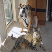
To understand more about the above two points, let us consider Figure 6 as the input to the VGG16 model, for which predictions are - "Bull_mastiff" with a probability of 0.24 and another relevant prediction is "Tiger_cat" with a probability of 0.073.

For the above image, the class discriminative visual explanation can be done by the GradCAM technique, which is shown in Figures 7 and 8.

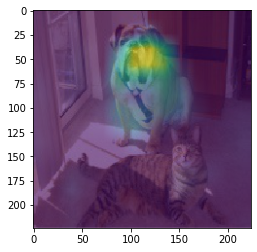
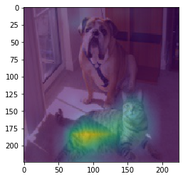
Here it is observed that for predicting image as "Bull_mastiff" model is mainly focusing on the face of bull_mastiff and for predicting image as "Tiger_cat" model is mainly focusing on the body part of the cat

In the case of fine-grained detail, it can be achieved by Guided Backpropagation which is shown in Figure 9.

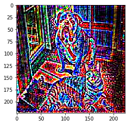
Guided Backpropagation only focuses on the positive influences which result in pixel-level details.

Combining both these techniques (i.e. GradCAM and Guided GradCAM) will result in combining major factors which are essential for visual explanations (i.e. class discriminative and high resolution) which can be observed in Figure 10 and Figure 11.

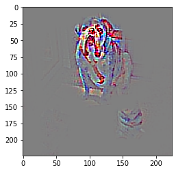
From Figure 11 it can be observed that "Tiger_cat" as prediction is mainly because of the stripes of the cat. Such high grained explanations can be achieved by Guided GradCAM

Conclusions

GradCAM is very much helpful for class discriminative explanation and Guided Backpropagation is helpful for explanation with higher resolutions. Combining both these techniques (i.e. Guided GradCAM) creates a more powerful explainability technique that can help analyze the model's predictions and retrain accordingly. Such explainability techniques will surely help increase the trust in the model and its predictions.

References

1. https://arxiv.org/abs/1610.02391
2. https://github.com/ismailuddin/gradcam-tensorflow-2
3. https://arxiv.org/abs/1611.07450

Also Checkout: One such magical product that offers explainability is AIEnsured by testAIng. Do check this link.