Artificial Intelligence / Machine Learning

Complete Journey of an ML Model

Aiensured

Nov 28, 2023 • 10 min read

This article on the journey of an ML model will take you through the entire process from when the model is built to where it can be used in a web container.

The journey starts with building the model, training it on a dataset, finetuning it, testing it, logging and tracking the training, deploying the model in a web container and also explaining how the model reached a particular prediction or decision.

In this article, the dandelion dataset is used to train the model.

Building and Training the Model:

First, the dataset is loaded from Kaggle and the images are labelled. Then the dataset is divided into training and test datasets. The images are generated where the training set is further divided into train and validation sets and then the images are preprocessed.

import numpy as np
import pandas as pd
from pathlib import Path
import os.path
import matplotlib.pyplot as plt
from sklearn.model_selection import train_test_split
import tensorflow as tf
from tensorflow.keras import layers
from tensorflow.keras.preprocessing.image import ImageDataGenerator
from sklearn.metrics import accuracy_score,f1_score
from google.colab import drive

drive.mount('/content/gdrive')

from google.colab import files
files.upload() #the kaggle.json file is uploaded

!pip install -q kaggle #installing kaggle
!mkdir -p ~/.kaggle #making a new directory
!cp kaggle.json ~/.kaggle/
!chmod 600 /root/.kaggle/kaggle.json
!kaggle datasets download -d coloradokb/dandelionimages #downloading the dataset

!unzip dandelionimages.zip #unzipping it

image_dir=Path('/content/Images') #defining the path to the directory
filepaths =list(image_dir.glob(r'**/*.jpg'))
labels =list(map(lambda x: os.path.split(os.path.split(x)[0])[1], filepaths)) #giving labels to the paths of the images
filepaths = pd.Series(filepaths, name='Filepath').astype(str)
labels = pd.Series(labels, name='Label')
image_df = pd.concat([filepaths, labels], axis=1) #concatinating the filepaths and the labels

train_df, test_df = train_test_split(image_df, train_size=0.7, shuffle=True, random_state=1)

train_generator = ImageDataGenerator( #generating the train data with 20% being validation set
preprocessing_function=tf.keras.applications.mobilenet_v2.preprocess_input,
validation_split=0.2
)
test_generator = ImageDataGenerator( #generating the test data
preprocessing_function=tf.keras.applications.mobilenet_v2.preprocess_input
)

train_images = train_generator.flow_from_dataframe(
dataframe=train_df,
x_col='Filepath',
y_col='Label',
target_size=(224, 224),
color_mode='rgb',
class_mode='binary',
batch_size=32,
shuffle=True,
seed=42,
subset='training'
)

val_images = train_generator.flow_from_dataframe(
dataframe=train_df,
x_col='Filepath',

y_col='Label',
target_size=(224, 224),
color_mode='rgb',
class_mode='binary',
batch_size=32,
shuffle=True,
seed=42,
subset='validation'
)

test_images = test_generator.flow_from_dataframe(
dataframe=test_df,
x_col='Filepath',
y_col='Label',
target_size=(224, 224),
color_mode='rgb',
class_mode='binary',
batch_size=32,
shuffle=False
)

The features of these images are then extracted. Then the model is built where the last layer is made sure to have a sigmoid function as it is a binary classification.

feature_extractor = tf.keras.applications.MobileNetV2( #extracting the features of the given images
input_shape=(224, 224, 3),
weights='imagenet',
include_top=False,
pooling='avg'
)

feature_extractor.trainable = False

inputs = feature_extractor.input #model
x = tf.keras.layers.Dense(128, activation='relu')(feature_extractor.output)
x = tf.keras.layers.Dense(128, activation='relu')(x)
outputs = tf.keras.layers.Dense(1, activation='sigmoid')(x) #sigmoid so that the outer layer gives 1 or 0 classifying the images

model = tf.keras.Model(inputs=inputs, outputs=outputs)

model.compile(
optimizer='adam',
loss='binary_crossentropy',
metrics=['accuracy']
)

print(model.summary())

The optimizer is chosen to be ‘Adam’ as this gave the highest accuracy

for the given epochs. The training is done for 10 epochs.

history = model.fit( #training the model
train_images,
validation_data=val_images,
epochs=10,
)

Epoch 1/10 23/23 [==============================] - 144s 6s/step - loss: 0.3262 - accuracy: 0.8402 - val_loss: 0.4542 - val_accuracy: 0.7670 Epoch 2/10 23/23 [==============================] - 146s 6s/step - loss: 0.2661 - accuracy: 0.8840 - val_loss: 0.4936 - val_accuracy: 0.8068 Epoch 3/10 23/23 [==============================] - 142s 6s/step - loss: 0.2949 - accuracy: 0.8656 - val_loss: 0.6041 - val_accuracy: 0.7614 Epoch 4/10 23/23 [==============================] - 151s 7s/step - loss: 0.2275 - accuracy: 0.9010 - val_loss: 0.3938 - val_accuracy: 0.8295 Epoch 5/10 23/23 [==============================] - 155s 7s/step - loss: 0.1434 - accuracy: 0.9491 - val_loss: 0.4632 - val_accuracy: 0.8409 Epoch 6/10 23/23 [==============================] - 156s 7s/step - loss: 0.1096 - accuracy: 0.9576 - val_loss: 0.3834 - val_accuracy: 0.8409 Epoch 7/10 23/23 [==============================] - 152s 7s/step - loss: 0.1303 - accuracy: 0.9448 - val_loss: 0.4142 - val_accuracy: 0.8239 Epoch 8/10 23/23 [==============================] - 143s 6s/step - loss: 0.1210 - accuracy: 0.9533 - val_loss: 0.4200 - val_accuracy: 0.8466 Epoch 9/10 23/23 [==============================] - 154s 7s/step - loss: 0.0942 - accuracy: 0.9661 - val_loss: 0.5142 - val_accuracy: 0.8409 Epoch 10/10 23/23 [==============================] - 152s 7s/step - loss: 0.0654 - accuracy: 0.9816 - val_loss: 0.4301 - val_accuracy: 0.8693

Now the model is tested with the test dataset for its accuracy.

predictions = np.squeeze(model.predict(test_images)) #vgg16 #resnet50
predictions = (predictions >= 0.5).astype(int)

acc = accuracy_score(test_images.labels, predictions)
f1 = f1_score(test_images.labels, predictions)

print("Accuracy: {:.2f}%".format(acc * 100))
print("F1-Score: {:.5f}".format(f1))

12/12 [==============================] - 71s 6s/step Accuracy: 86.02% F1-Score: 0.86016

model.save('/content/Images/model.h5')

Then the model is saved in the directory for further use.

This classification is also done using pre-trained models like resnet50 and vgg16.

Resnet50:

from tensorflow.keras.applications import ResNet50
from tensorflow.keras.layers import Dense, GlobalAveragePooling2D
from tensorflow.keras.models import Model # Load the ResNet-50 model (pretrained on ImageNet)
base_model = ResNet50(weights='imagenet', include_top=False, input_shape=(224, 224, 3)) # Add custom layers on top of the pretrained model
x = base_model.output
x = GlobalAveragePooling2D()(x)
x = Dense(128, activation='relu')(x)
predictions = Dense(1, activation='sigmoid')(x)

model = Model(inputs=base_model.input, outputs=predictions) # Freeze the pretrained layers
for layer in base_model.layers:
layer.trainable = False # Compile the model
model.compile(optimizer='adam',
loss='binary_crossentropy',
metrics=['accuracy']) # Train the model
model.fit(
train_images,
validation_data=val_images,
epochs=10
)

The training accuracy with resnet50 was 73.8% and the validation accuracy was 68.75%.

Vgg16:

from tensorflow.keras.applications import VGG16
from tensorflow.keras.layers import Dense, Flatten # Load the VGG16 model (pretrained on ImageNet)
base_model = VGG16(weights='imagenet', include_top=False, input_shape=(224, 224, 3)) # Add custom layers on top of the pretrained model
x = base_model.output
x = Flatten()(x)
x = Dense(128, activation='relu')(x)
predictions = Dense(1, activation='sigmoid')(x)

model = Model(inputs=base_model.input, outputs=predictions) # Freeze the pretrained layers
for layer in base_model.layers:
    layer.trainable = False # Compile the model
model.compile(optimizer='adam',
              loss='binary_crossentropy',
              metrics=['accuracy']) # Train the model
model.fit(
    train_images,
    validation_data=val_images,
    epochs=10
)

The training accuracy with vgg16 was 88.9% and the validation accuracy was 77.84% (which is more than resnet50).

The custom model had the highest accuracy of the three models.

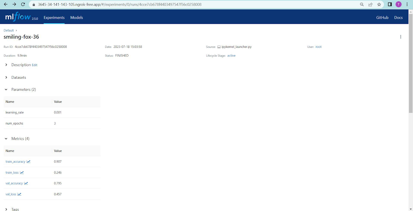
Logging and Tracking with ML Flow:

The parameters and the metrics are logged in the ml flow UI. By setting a tracking Uri the model can be tracked while training.

import numpy as np
import pandas as pd
from pathlib import Path
import os.path
!pip install mlflow #installing mlflow

from sklearn.model_selection import train_test_split
from tensorflow.keras.preprocessing.image import ImageDataGenerator
import tensorflow as tf
from sklearn.metrics import accuracy_score, f1_score

import mlflow
mlflow.set_tracking_uri("file:/content/mlruns") #setting the trackinh uri

The below code is used for logging the parameters and tracking the model.

mlflow.start_run() # Start MLflow run

learning_rate = 0.001
num_epochs = 3
mlflow.log_param("learning_rate", learning_rate)
mlflow.log_param("num_epochs", num_epochs) # Log the model architecture
model.summary()
model_architecture_path = "model_architecture.png"
tf.keras.utils.plot_model(model, to_file=model_architecture_path, show_shapes=True)
mlflow.log_artifact(model_architecture_path)

( The above code is run just after building the model and the below one is run after training)

mlflow.log_metric("train_accuracy", history.history["accuracy"][-1]) # Log metrics
mlflow.log_metric("val_accuracy", history.history["val_accuracy"][-1])
mlflow.log_metric("train_loss", history.history["loss"][-1])
mlflow.log_metric("val_loss", history.history["val_loss"][-1]) # Save the trained model
model.save('/content/Images/model.h5')
mlflow.tensorflow.log_model(model, "model")
mlflow.end_run() # End the MLflow run

Using pyngrok the ml flow ui is accessed from colab.

!pip install pyngrok
from pyngrok import ngrok #connecting to the mlflow ui using ngrok
ngrok.set_auth_token("your auth token") #replace it with your authorization token
ngrok.connect(5000)
!mlflow ui --host 0.0.0.0

The ml flow UI looks like this.

Explaining the model with the XRAI explainability technique:

This section discusses the technique used for explaining why and how the model predicted the image. It also shows areas and parameters were important for that prediction.

XRAI stands for eXplainable Reverse Attention for Image classification. It is a technique which shows visually the areas that were important for making a prediction using a heatmap and integrated gradients. The entire process involves several steps - preprocessing the images, calculating integrated gradients, the images are segmented, attributions are calculated and aggregated with the segments, the segments are ranked based on the attributions, the heatmap is generated according to the ranks and overlaid on the original image to find the important areas.

import cv2
import numpy as np
import matplotlib.pyplot as plt
from skimage.segmentation import felzenszwalb
def integrated_gradients(input_image, model, baseline_image, num_steps=50):# Calculate the gradients with respect to the input image
gradients = []
img_gradients = tf.zeros_like(input_image)
for step in range(num_steps + 1):
alpha = step / num_steps
interpolated_image = baseline_image + alpha * (input_image - baseline_image)
interpolated_image = tf.clip_by_value(interpolated_image, 0.0, 1.0)
with tf.GradientTape() as tape:
tape.watch(interpolated_image)
logits = model(interpolated_image)
top_prediction = tf.argmax(logits, axis=1)
grads = tape.gradient(logits, interpolated_image)

if grads is not None:
img_gradients += grads / num_steps
else:
print("Gradients are None.")

return img_gradients

def aggregate_attributions(input_image, segments, attributions):
num_segments = np.max(segments) + 1
aggregated_attributions = np.zeros(num_segments) # Sum up attributions within each segment
for segment_id in range(num_segments):
mask = segments == segment_id
segment_attributions = attributions * mask[..., np.newaxis]
aggregated_attributions[segment_id] = np.sum(segment_attributions)

return aggregated_attributions

def rank_segments(aggregated_attributions):
ranked_segments = np.argsort(aggregated_attributions)[::-1]
return ranked_segments

def generate_heatmap(input_image, segments, ranked_segments):
heatmap = np.zeros_like(input_image) # Color the top-ranked segments in the heatmap
for segment_id in ranked_segments:
mask = segments == segment_id
heatmap += mask[..., np.newaxis] * input_image

return heatmap

nput_image = cv2.imread("/content/Images/dandelion/IMG_5421.jpg") # Check if the image is loaded successfully
if input_image is not None: # Resize the input image to match the expected input shape
input_image = cv2.resize(input_image, (224, 224)) # Convert the input image to a float32 array
input_image = input_image.astype(np.float32) # Normalize the pixel values to a range of [0, 1]
input_image /= 255.0 # Add a batch dimension
input_image = np.expand_dims(input_image, axis=0)

else:
print("Failed to load the input image.") # Define a baseline image (e.g., all black or white image)
baseline_image = np.zeros_like(input_image) # Calculate the pixel-level attributions using Integrated Gradients
attributions = integrated_gradients(input_image, model, baseline_image, num_steps=50) # Apply Felzenszwalb's graph-based segmentation
segments = felzenszwalb(input_image[0], scale=250, sigma=0.8, min_size=50) # Aggregate attributions within segments
aggregated_attributions = aggregate_attributions(input_image[0], segments, attributions) # Rank the segments
ranked_segments = rank_segments(aggregated_attributions) # Generate the heatmap
heatmap = generate_heatmap(input_image[0], segments, ranked_segments) # Apply the colormap to the heatmap
heatmap_colormap = cv2.applyColorMap(np.uint8(255 * heatmap), cv2.COLORMAP_JET)

heatmap_colormap = heatmap_colormap.astype(input_image.dtype) # Overlay the heatmap on the original image
alpha = 0.6
beta = 0.4
overlay = cv2.addWeighted(input_image[0], alpha, heatmap_colormap, beta, 0)

plt.figure(figsize=(10, 6))

plt.subplot(1, 3, 1)
plt.imshow(cv2.cvtColor(input_image[0], cv2.COLOR_BGR2RGB))
plt.title('Original Image')
plt.axis('off')

plt.subplot(1, 3, 2)
plt.imshow(heatmap, cmap='hot')
plt.title('Heatmap')
plt.axis('off')

plt.subplot(1, 3, 3)
plt.imshow(cv2.cvtColor(overlay, cv2.COLOR_BGR2RGB))
plt.title('Original Image with Heatmap')
plt.axis('off')

plt.show()

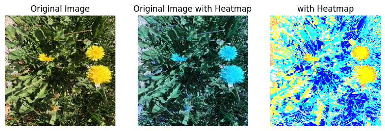
The areas in yellow are the important areas that lead to the prediction.

There are many other methods that show visually the important areas like the above technique and any one of them can be used to understand the model better.

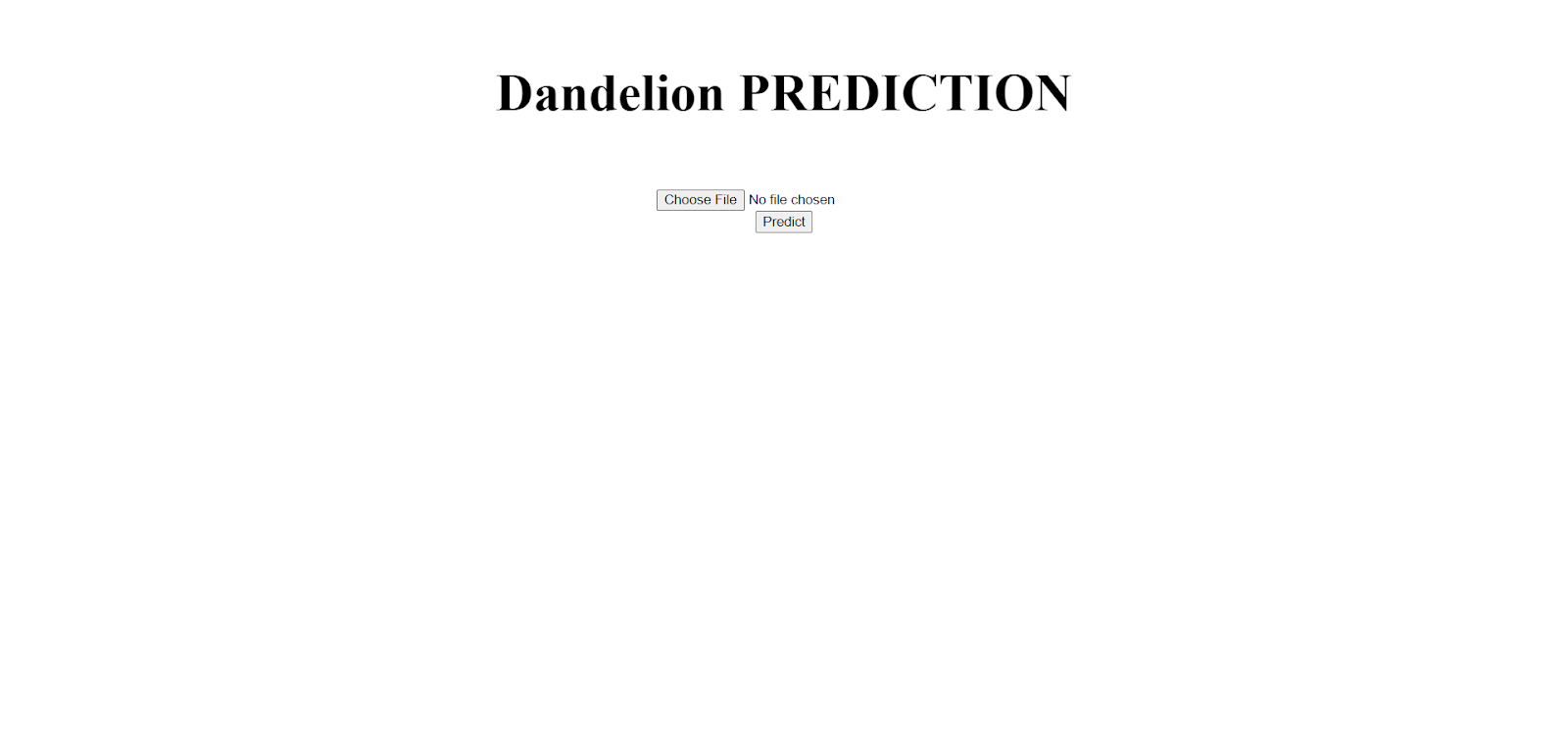
Deploying the model in a web container using Flask:

Using Flask the model is deployed such that it can be used in a web container. As it is implemented in Google Colab, the website URL (after deployment) is made public using Pyngrok as it cannot access the local host being a cloud-based platform.

HTML file:

%%writefile home.html

Dandelion Prediction

Dandelion PREDICTION

{% if prediction %}

Prediction: {{ prediction }}

{% endif %}

The HTML file is given in this format and not as an HTML template as Google Colab doesn't support template rendering.

import os
import flask
from flask import send_file
import PIL.Image
import numpy as np
import pyngrok
import tensorflow as tf
from tensorflow.keras.preprocessing.image import img_to_array
from tensorflow.keras.applications.mobilenet_v2 import preprocess_input
from pyngrok import ngrok

model = tf.keras.models.load_model('/content/Images/cnn-model.h5')
app = flask.Flask(name)

@app.route('/')
def home2():
return send_file('home.html')

@app.route('/predict', methods=['POST'])
def predict():

file = flask.request.files['image'] # Get the image from the request
img_path = "/content/temp.jpg"
file.save(img_path)

img = PIL.Image.open(img_path)
img = img.resize((224, 224)) # Resize the image to (224, 224) # Load and preprocess the image

img_array = img_to_array(img) # Convert the PIL Image object to a NumPy array

img_array = np.expand_dims(img_array, axis=0)# Add a batch dimension and preprocess the image
img_array = preprocess_input(img_array)

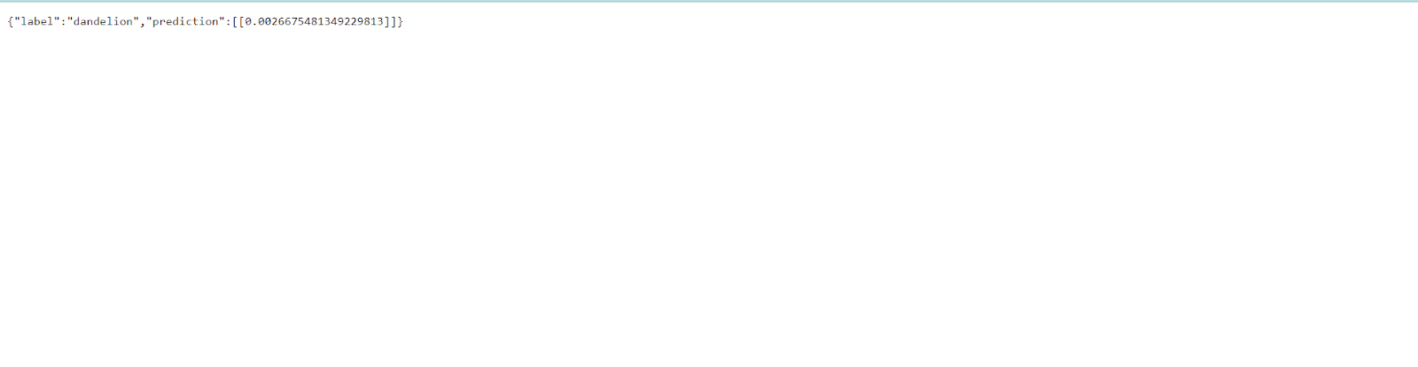
prediction = model.predict(img_array)# Make the prediction

predicted_class = np.argmax(prediction) # Get the class label with the highest probability

probability = prediction[0][predicted_class] # Get the probability of the predicted class

threshold = 0.5 # Define a threshold to differentiate between dandelion and other

if probability >= threshold: # Assign the label based on the probability and the threshold
label = "other"
else:
label = "dandelion"

prediction_list = prediction.tolist()# Convert the NumPy array to a Python list for JSON serialization

img_processed = PIL.Image.fromarray(np.squeeze(img_array, axis=0).astype(np.uint8), 'RGB') # Show the image after it is processed (optional)
img_processed.show()

return flask.jsonify({'prediction': prediction_list, 'label': label})# Return the prediction result as JSON along with the label

ngrok.set_auth_token('your auth token')# Set the ngrok auth token

ngrok_tunnel = ngrok.connect(addr="5000", bind_tls=True)# Connect using pyngrok without specifying the region

public_url = ngrok_tunnel.public_url # Get the public URL
print("Public URL:", public_url)

app.run(host="0.0.0.0", port=5000) # Start the Flask app

The above code gives the public URL as the output along with the debug status and on which server it is running. It is a developmental server in this case. It also gives the preprocessed images in the colab.

In this case, the prediction is such that if the prediction score is nearer to 0 then it is labelled as a dandelion image and if it is nearer to 1 it is labelled as other (not a dandelion).

The static HTML page looks like this: