Cracking the Kernel: Interactive Insights into Support Vector Machines

Introduction:
Support Vector Machines (SVMs) have emerged as powerful and versatile machine learning algorithms with applications ranging from classification to regression. SVMs excel at finding optimal decision boundaries in complex data spaces, thanks to their ingenious use of kernels. In this interactive article, we will delve into the world of SVMs, uncover the secrets behind their success, and explore the fascinating role of kernels in SVMs.
Understanding SVMs:
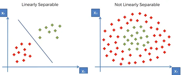
In this section, we will introduce the basic concepts of SVMs, including the notion of maximum margin classifiers. We will explain the intuition behind SVMs, their ability to handle both linearly separable and non-linearly separable data, and their unique approach to finding the optimal decision boundary.
The Kernel Trick:
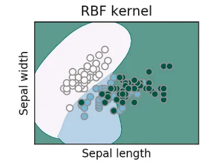
The kernel trick lies at the heart of SVMs and is responsible for their remarkable ability to handle complex, non-linear datasets. We will take an interactive journey through various kernel functions, such as linear, polynomial, and radial basis function (RBF), and explore their impact on SVM performance
Kernel Selection Strategies:
Choosing an appropriate kernel function is crucial for achieving good SVM performance. We will explore various strategies for kernel selection, including domain expertise, empirical evaluation, and hyperparameter tuning. Interactive examples and case studies will highlight the strengths and weaknesses of different kernel functions in different scenarios.
1. The Intuition:
At its core, an SVM aims to find the optimal hyperplane that best separates data points of different classes. The term "support vector" refers to the data points that lie closest to the decision boundary. These vectors play a crucial role in the SVM algorithm, as they define the position and orientation of the separating hyperplane.
2. Linear SVM:
Let's start with the case of linear SVMs, where the decision boundary is a straight line in a two-dimensional space. To achieve the best separation, we want the hyperplane with the maximum margin, which is the distance between the hyperplane and the closest data points from each class.
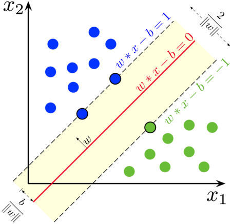
We have taken the distance between in both support vectors as 2
3. Maximizing the Margin:
Given a training dataset with input vectors (X) and corresponding class labels (Y), we want to find a hyperplane defined by the equation w⋅x + b = 0, where w represents the weights and b is the bias term. We introduce the concept of functional margin, which is defined as Yi * (w⋅xi + b) for each training example (xi, Yi). The goal is to find the optimal w and b that maximize the functional margin.

Is called as functional margin
4. Optimization Objective:
To formulate the optimization objective, we introduce the concept of geometric margin, which is the functional margin divided by the magnitude of the weight vector, ||w||. Thus, the geometric margin for any point (xi, Yi) can be calculated as Yi * ((w⋅xi + b) / ||w||).
5. Optimization Problem:
Formally, the optimization problem can be stated as follows: maximize the geometric margin subject to the constraint that Yi * ((w⋅xi + b) / ||w||) ≥ 1 for all training examples (xi, Yi). This constraint ensures that all data points are classified correctly and lie on the correct side of the decision boundary.
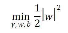
By following the above equations and solve it using geometry we can finally get a condition which says to minimize the ||w||
6. Convex Optimization:
Solving the optimization problem involves minimizing the objective function, which is equivalent to minimizing the ||w||^2. This leads to a convex optimization problem that can be efficiently solved using techniques such as Quadratic Programming.

Quadratic programming :
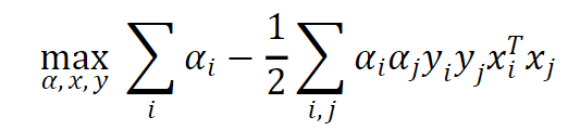
In SVMs, the objective function of the optimization problem involves minimizing the ||w||^2, subject to the constraints Yi * ((w⋅xi + b) / ||w||) ≥ 1 for all training examples (xi, Yi). This objective function is quadratic, while the constraints are linear. Therefore, it is a quadratic programming problem:
To solve the QP problem in SVMs, specialized algorithms and solvers are utilized. These solvers aim to find the optimal values for w and b that satisfy the constraints and minimize the quadratic objective function.
SVMs use the concept of Lagrange multipliers. Lagrange multipliers introduce a set of variables (αi) associated with each training example, which represent the weights assigned to the constraints. These Lagrange multipliers allow the SVM to handle nonlinear boundaries by implicitly transforming the data into a higher-dimensional feature space.
But in programming computer uses complex methods to give the ideal values of the W and b. But the basis are as follows
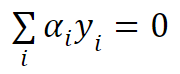
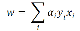
We find the corresponding value of αi for each xi in the dataset(train) and set the value of wi using the below equation:
7. Soft Margin SVM:
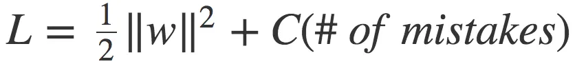
In real-world scenarios, the data may not be perfectly separable by a hyperplane. To handle such cases, we introduce the concept of a soft margin. The soft margin SVM allows for a certain degree of misclassification by introducing slack variables, which penalize misclassified points. This leads to a more robust and flexible model.
8. Nonlinear SVM:
In many cases, a linear decision boundary is not sufficient to separate complex data. SVMs address this limitation by using the kernel trick. The kernel function enables SVMs to implicitly map the data into a higher-dimensional feature space, where a linear decision boundary can be found. Common kernel functions include the linear, polynomial, radial basis function (RBF), and sigmoid kernels.


Conclusion:
Support Vector Machines (SVMs) are fascinating models that leverage elegant mathematical concepts to achieve accurate and robust classification and regression. By maximizing the margin between classes, SVMs find the optimal hyperplane that best separates data points. Their flexibility extends to nonlinear problems through the kernel trick. Understanding the mathematics behind SVMs not only sheds light on their inner workings but also enables us to appreciate the effectiveness of these models
Do Checkout:
Explore our other articles do check at https://blog.aiensured.com/
By S.B.N.V.Sai Dattu