Customer Segmentation Classification (Part-2)

Hyper parameter tuning and cross-validation

To cook your favourite dish, you know to set the oven to 180 degrees and turn the grill on. But when your roommate cooks their favourite dish, they set use 200 degrees and the fan-forced mode. Same oven, different settings, different outcomes.
The same can be done for machine learning algorithms. You can use the same algorithms but change the settings (hyperparameters) and get different results.
But just like turning the oven up too high can burn your food, the same can happen for machine learning algorithms. You change the settings and it works so well, it overfits (does too well) the data.

We're looking for the goldilocks model. One which does well on our dataset but also does well on unseen examples.

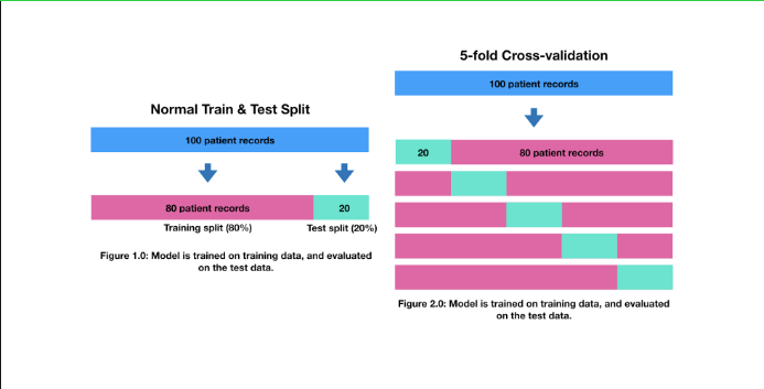
To test different hyper-parameters, you could use a validation set but since we don't have much data, we'll use cross-validation.

The most common type of cross-validation is k-fold. It involves splitting your data into k-fold's and then testing a model on each. For example, let's say we had 5 folds (k = 5). This what it might look like.

Hyperparameter types

In logistic regression, hyperparameters are parameters that are set before the model is trained and can significantly influence the model's performance. The main hyperparameters that we can tune in logistic regression, along with their descriptions, are as follows:

1. Solver: The solver is an optimization algorithm used to find the optimal weights for logistic regression. Different solvers have different computational properties, and the choice of solver can impact the convergence speed and memory usage. The available choices are:

  - 'lbfgs': This solver is a good default choice and generally performs well on a wide range of problems while saving memory. However, it may have convergence issues in some cases.

   - 'sag': This solver is faster for large datasets, particularly when both the number of samples and features are large. It can be beneficial for large-scale problems.

  - 'saga': This solver is well-suited for sparse multinomial logistic regression and is suitable for very large datasets.

  - 'newton-cg': This solver can be computationally expensive due to the Hessian Matrix, which is required for its optimisation process.

 - 'liblinear': This solver is recommended for high-dimensional datasets and is effective for large-scale classification problems.

2. Penalty: The penalty is a regularisation term added to the loss function to prevent overfitting. It helps to control the complexity of the model. The available choices are 'l1' and 'l2', referring to L1 (Lasso) and L2 (Ridge) regularization, respectively.

3. C (Regularisation Strength): The inverse of the regularisation strength, C, determines how much to penalize large coefficients. Smaller values of C increase the regularization strength, leading to simpler models.

4. Max_iter: This hyperparameter sets the maximum number of iterations allowed for the solver to converge to an optimal solution. If the solver does not converge within this limit, it may terminate prematurely without finding the best weights.

To achieve better performance and convergence, especially for 'sag' and 'saga' solvers, it is recommended to scale the data using either `StandardScaler` or `MinMaxScaler` from the `sklearn.preprocessing` module before fitting the logistic regression model. Scaling ensures that features have similar scales, which can help the solvers converge faster and more accurately.

Random Forest is an ensemble learning algorithm that combines multiple decision trees to create a more robust and accurate model. In a Random Forest, there are several hyperparameters that can be controlled to influence the construction of individual decision trees and the overall behavior of the forest. Let's explain each of these hyperparameters:

1. n_estimators: The number of decision trees being built in the Random Forest. Increasing the number of estimators typically improves the model's performance and makes it more robust. However, a large number of trees can lead to longer training times.

2. criterion: The function used to measure the quality of splits in a decision tree during the tree-building process. For classification problems, you can choose between 'gini' (Gini impurity) and 'entropy' (information gain). For regression problems, you can use 'mse' (Mean Squared Error) or 'mae' (Mean Absolute Error). The criterion determines how the decision tree finds the best split at each node.

3. max_depth: The maximum levels allowed in a decision tree. By setting a maximum depth, you control the complexity of individual decision trees. Too deep trees can overfit, while shallow trees may not capture complex patterns in the data.

4. max_features: The maximum number of features considered when looking for the best split at a node. By limiting the number of features, the algorithm introduces more randomness and diversity into the forest. Common choices are 'sqrt' (square root of the total number of features) or 'log2' (logarithm base 2 of the total number of features).

5. bootstrap: A boolean parameter that determines whether bootstrap samples are used to build individual decision trees. If True, each tree is trained on a random subset of the data (with replacement), making the trees slightly different and promoting diversity.

6. min_samples_split: The minimum number of samples required to split an internal node. This parameter controls the stopping criteria for the splitting process. If the number of samples in a node is less than the specified value, further splitting is stopped, reducing the risk of overfitting.

7. min_samples_leaf: The minimum number of samples required to be at a leaf node. It helps control the depth of the tree and prevents overfitting. If a split results in a node with fewer samples than the specified value, the split is cancelled.

8. max_leaf_nodes: By setting this hyperparameter, you can limit the number of leaf nodes in the decision tree. It effectively restricts the growth of the tree, preventing overfitting and making the tree more interpretable.

Since SVMs is suitable for small data set: the SVM model would be good with high accuracy expect using Sigmoid kernels. We could be able to determine which kernel performs the best based on the performance metrics such as precision, recall and f1 score.

In order to improve the model accuracy, there are several parameters need to be tuned. Three major parameters including:

• Kernels: The main function of the kernel is to take low dimensional input space and transform it into a higher-dimensional space. It is mostly useful in non-linear separation problem.

• C (Regularisation): C is the penalty parameter, which represents misclassification or error term. The misclassification or error term tells the SVM optimisation how much error is bearable. This is how you can control the trade-off between decision boundary and misclassification term.

• when C is high it will classify all the data points correctly, also there is a chance to overfit.
• 3. Gamma: It defines how far influences the calculation of plausible line of separation.

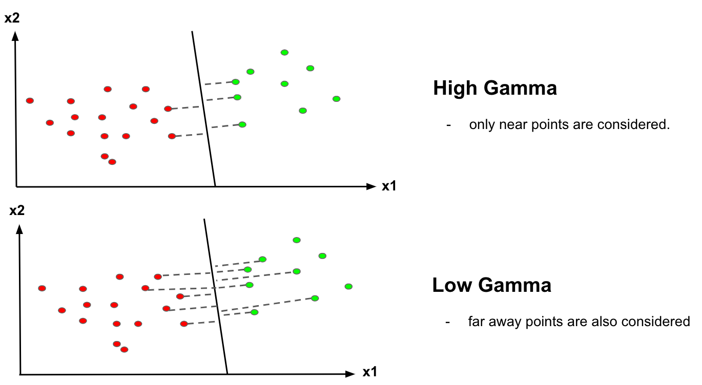
when gamma is higher, nearby points will have high influence; low gamma means far away points also be considered to get the decision boundary.

Methods for tuning hyperparameters

Now that we understand what hyperparameters are and the importance of tuning them, we need to know how to choose their optimal values. We can find these optimal hyperparameter values using manual or automated methods.

When tuning hyperparameters manually, we typically start using the default recommended values or rules of thumb, then search through a range of values using trial-and-error. But manual tuning is a tedious and time-consuming approach. It isn’t practical when there are many hyperparameters with a wide range.

Automated hyperparameter tuning methods use an algorithm to search for the optimal values. Some of today’s most popular automated methods are grid search, random search, and Bayesian optimization. Let’s explore these methods in detail.

Grid search

Grid search is a sort of “brute force” hyperparameter tuning method. We create a grid of possible discrete hyperparameter values then fit the model with every possible combination. We record the model performance for each set then select the combination that has produced the best performance.

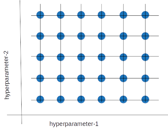
Grid search is a hyperparameter tuning method in which we create a grid of possible discrete hyperparameter values, then fit the model with every possible combination.

Grid search is an exhaustive algorithm that can find the best combination of hyperparameters. However, the drawback is that it’s slow. Fitting the model with every possible combination usually requires a high computation capacity and significant time, which may not be available.

Random search

The random search method (as its name implies) chooses values randomly rather than using a predefined set of values like the grid search method. 

Random search tries a random combination of hyperparameters in each iteration and records the model performance. After several iterations, it returns the mix that produced the best result.

Random search tries a random combination of hyperparameters in each iteration and records the model performance. After several iterations, it returns the mix that produced the best result.

Random search is appropriate when we have several hyperparameters with relatively large search domains. We can make discrete ranges (for instance, [5-100] in steps of 5) and still get a reasonably good set of combinations.

The benefit is that random search typically requires less time than grid search to return a comparable result. It also ensures we don't end up with a model that's biased toward value sets arbitrarily chosen by users. Its drawback is that the result may not be the best possible hyperparameter combination.

Model Explainability

Model explainability refers to the ability of a machine learning model to provide understandable and interpretable insights into its decision-making process. When a model is deployed for real-world use, it is crucial for model developers and stakeholders, such as domain experts and end-users, to comprehend how the model arrives at its predictions or classifications.

In scenarios like healthcare, where decisions based on the model's predictions can have significant consequences, understanding the factors and features that influence the model's output is of utmost importance. Explainability enables medical practitioners and domain experts to gain insights into the model's reasoning, identify which features are considered important, and uncover potential biases or inconsistencies in the model's behavior.

Essentially, model explainability involves answering questions like

• Which input features or parameters are the most influential in the model's decision?
• How does the model use these features to make predictions or classifications?
• Are there any patterns or trends that the model relies on to reach specific conclusions?
• Are there any particular instances where the model performs exceptionally well or poorly, and why?
• Are there any factors that might introduce biases or unfairness in the model's predictions?

Developing model understanding can be achieved through two approaches:

Option 1:Glass Box Models: In this approach, models are chosen or designed to be inherently interpret able. Linear regression is a classic example of an interpretable model, where the coefficients directly reveal the impact of each input feature on the output. Such models provide clear insights into the relationship between the input variables and the predictions.

Option 2: Black Box Models: In this approach, complex models, often referred to as black box models, are trained to achieve high predictive performance but lack inherent interoperability. After building these models, post-hoc explanation techniques are used to understand their decision-making process. Techniques like SHAP (SHapley Additive exPlanations) or LIME (Local Interpretable Model-agnostic Explanations) help provide insights into how the model arrives at its predictions for specific instances.

Global Interpretation
Global interpretation techniques aim to provide a holistic understanding of the model's behavior across the entire dataset. These techniques help identify the overall trends, patterns, and feature importances that the model considers for making predictions.

1. Feature Importance: As mentioned earlier, feature importance analysis is a global interpretation technique that ranks the input features based on their impact on the model's predictions. It helps identify the most influential features across the entire dataset.

2. Partial Dependence Plots (PDP): PDP provides a global view of how individual features influence the model's predictions by averaging the effects over the entire dataset. It shows the average relationship between each feature and the predicted outcome.

3. Accumulated Local Effects (ALE) Plots: ALE plots visualize the cumulative contributions of each feature to the model's predictions across the dataset. It provides insights into how each feature impacts the model's predictions when considered together.

4. Global Surrogate Models: In cases where the original model is a complex black box model, global surrogate models (e.g., linear models) can be built to approximate the behaviour of the black box model. Surrogate models offer a more interpretable representation of the original model's decision boundaries and feature importance.

Local Interpretation:

Local interpretation techniques aim to explain the model's predictions for individual instances or a small group of instances. These techniques provide insights into why the model made specific decisions for particular data points.

1. Individual Conditional Expectation (ICE) Plots: ICE plots, as mentioned earlier, offer local interpretations by showing the predictions for individual instances as the value of one feature changes while keeping other features constant.

2. Local Interpretable Model-agnostic Explanations (LIME): LIME is a popular method for providing local interpretations for black box models. It creates interpretable surrogate models for individual instances and approximates how the black box model behaves around the prediction of interest.

3. SHAP (SHapley Additive exPlanations): SHAP values can be used for both global and local interpretation. For local interpretation, SHAP values provide the contribution of each feature to the difference between the model's prediction for a specific instance and the average prediction.

The combination of global and local interpretation techniques provides a comprehensive understanding of the model's behavior, allowing stakeholders to validate its predictions, detect biases, and ensure transparency and accountability in the decision-making process.

Basic Hands-on learning model explainability methods

Here we are going to explain our model using Lime, to do that we have to first install lime in our system.
pip install lime

import lime
import lime.lime_tabular
import pandas as pd

Assuming X_test is a NumPy array

X_test_df = pd.DataFrame(X_test, columns=X_features)

explainer = lime.lime_tabular.LimeTabularExplainer(
training_data=X_train,
training_labels=Y_train,
feature_names=X_features,
discretize_continuous=True,
class_names=['A','B','C','D'],
kernel_width=3,
verbose=True,
mode = 'classification'
)

Now you can use .iloc to access the first row of X_test_df

X_test_df.iloc[0]
exp = explainer.explain_instance( X_test_df.iloc[0],
rs_rf.predict_proba )

Intercept 0.3164447201816717
Prediction_local [0.15976574]
Right: 0.1539384739832546

exp.show_in_notebook(show_table=True, show_all=True)
Above line will show you a description about on which basis prediction is made.

For First part click here

For Third Part click here

References:

Written by - Ankit Mandal