Model Evaluation Metrics

Evaluation Metrics are quantitative measures that are used to assess the performance of a statistical or machine-learning model. These metrics provide insights as to how well the model is performing and help in comparing different models and algorithms. 

There are two types of models, regression model (continuous output) and classification model (nominal or binary output). The evaluation metrics used in each model are different.

The different evaluation methods for classification models are:

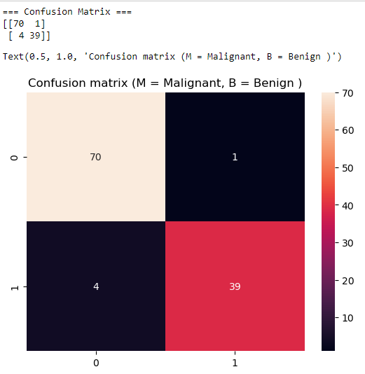
1. Confusion matrix: it is a matrix representation of the prediction results of any binary testing that is often used to describe the performance of the classification model on a set of test data for which true values are known. It is a N x N matrix, where N is the number of predicted classes. 

Each prediction can be one of the four outcomes, based on how it matches up to the actual value:

1. True positive (TP): Predicted True and true in reality
2. True negative (TN): Predicted False and False in reality
3. False positive (FP) (Type 1 Error): Predicted True and False in reality
4. True negative (FN) (Type 2 Error): Predicted False and True in reality

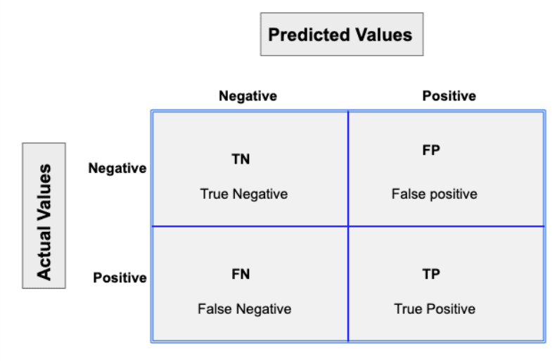
The diagonal elements represent the number of points for which the predicted label is equal to the true label, while anything off the diagonal is mislabeled. 

2. Accuracy: it is the most common evaluation metric for classification problems. It is the number of correct predictions made as a ratio of all predictions made. It can be calculated by using the formula:

Accuracy = (TP + TN)/ total 

3. Precision: it is an evaluation metric used to assess the performance of a classification model, particularly in scenarios where the focus is on minimizing false positives. It measures the proportion of correctly predicted positive instances out of all instances predicted as positives. Precision can be calculated using the formula:

Precision: TP/ (TP + FP)

4. Recall: also known as sensitivity or true positive rate, measures the proportion of correctly predicted positive values out of all the actual positive instances. It can be calculated by using the formula:

Recall: TP/ (TP + FN) 

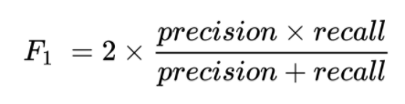
5. F1 Score: it is the harmonic mean of precision and recall, where the F1 score reaches the best value at 1 (perfect precision and recall) and the worst at 0. Since the harmonic mean of a list of numbers skews strongly toward the least elements of the list, it tends (compared to the arithmetic mean) to mitigate the impact of large outliers and aggravate the impact of small ones. If a model achieves high precision but low recall, it means it can accurately identify positive instances but may miss some positive instances, and vice versa. The F1 score balances these two aspects to provide an overall measure of the model’s performance.

The classification report combining precision, recall, and f1 score

6. Cross Validation: it involves partitioning the available dataset into multiple subsets, performing model training and evaluation on these subsets, then aggregating the results to estimate the model’s performance on unseen data. It repeatedly splits the original dataset into training and testing subsets. This helps to mitigate the potential bias and variance issues that can arise from relying on a single train-test split.
7. K - Fold Cross Validation: it is a resampling technique that estimates how well the model will perform on unseen data by simulating the process of training and evaluating the model on multiple subsets of available data. It splits the dataset into K subsets, each of equal size. The model is then trained on K-1 folds and evaluated on the remaining folds. The process is repeated K times, each time using a different fold for evaluation. The performance results from K iterations are averaged to obtain a single performance metric that represents the model’s overall performance. 

The different evaluation methods for regression models are:

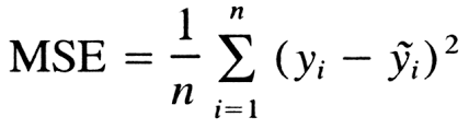
1. Mean Squared Error (MSE): it measures the amount of error in the models. It is the average squared difference between actual and predicted values. Squaring the differences eliminates negative values for the differences and ensures that the mean squared error is always greater than or equal to zero. Squaring increases the impact of larger errors. These calculations disproportionately penalize larger errors more than smaller errors. This property is essential when you want your model to have smaller errors.

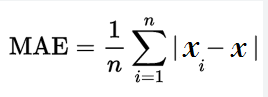
2. Mean Absolute Error (MAE):  it is measured by taking the absolute difference between the actual and predicted values, and then averaging it. It gives equal weight to all errors regardless of their direction (positive or negative), making it less sensitive to outliers compared to other metrics like Mean Squared Error.

3. Root Mean Squared Error (RMSE): it is the most common evaluation metric used in regression models. It is calculated by taking the square root of the Mean Squared Error. It follows an assumption that errors are unbiased and follow a normal distribution. The power of the square root empowers this metric to show a large number of deviations. It avoids the use of absolute errors, which is highly undesirable in calculations. As compared to Mean Absolute Error, RMSE gives higher weightage and punishes large errors. 

References:

https://www.analyticsvidhya.com/blog/2019/08/11-important-model-evaluation-error-metrics/

https://www.kdnuggets.com/2020/05/model-evaluation-metrics-machine-learning.html

https://statisticsbyjim.com/regression/mean-squared-error-mse/

By Arushi Paliwal