End-to-End Engine Horsepower Prediction with Deep Learning Regression Part-II

Introduction:

After completion of data preprocessing, we need to do the following steps to build the regression model.

1. Divide the Data into the Training and Test Sets.
2. Creating and Training a Neural Network with TensorFlow 2.0
3. Evaluating Neural Networks Performance

• Divide the Data into the Training and Test Sets:
  i) The task is to predict the efficiency of fuel based on the values in the other columns.
  ii) This is a regression problem because the predicted value is a regression value.
  iii) For predicting a regression value, we need to divide the dataset into training and test sets.

X = dataset.drop(['Horsepower'], axis=1)
y = dataset['Horsepower']
X_train, X_test, y_train, y_test=train_test_split(X,
y, test_size=0.2, random_state=20)

It is always a good practice to scale or standardize your data before training your artificial neural network on it. The following script applies to scale to the training and test sets:

from sklearn.preprocessing import StandardScaler
from sklearn.preprocessing import Normalizer
scaler = StandardScaler()
X_train = scaler.fit_transform(X_train)
X_test = scaler.transform(X_test)

• Creating and Training a Neural Network with TensorFlow 2.0:
  The next step is to create a neural network with TensorFlow 2.0. To do so, you first need to import the following libraries:

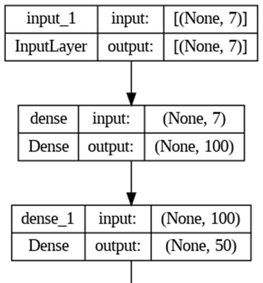
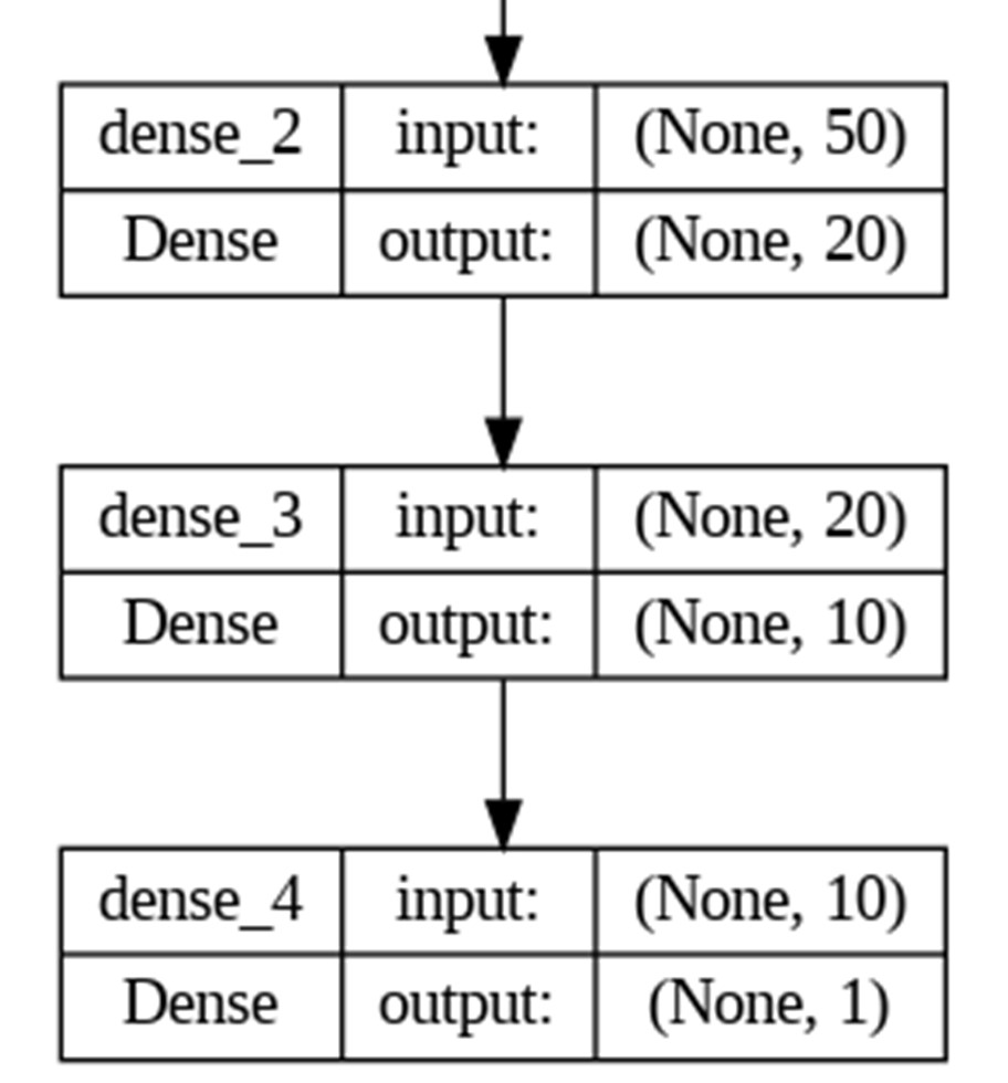
Next, we define a neural network with one input layer, 4 dense layers, and one output layer, run the following script. You can add or remove any layers if you want.

from tensorflow.keras.layers import Input, Dense,Activation,Dropout
from tensorflow.keras.models import Model
ip_layer = Input(shape=(X.shape[1],))
dl1 = Dense(100, activation='relu')(ip_layer)
dl2 = Dense(50, activation='relu')(dl1)
dl3 = Dense(20, activation='relu')(dl2)
dl4 = Dense(10, activation='relu')(dl3)
output = Dense(1)(dl4)

Finally, to create a neural network model using the layered architecture that you defined in the last step, execute the following script:

model = Model(inputs = ip_layer, outputs=output)
model.compile(loss="mean_absolute_error" , optimizer="adam", metrics=["mean_absolute_error"])

To plot the architecture of your neural network model, run the following script:

from keras.utils import plot_model
plot_model(model,to_file='model_plot.png',show_shapes=True,show_layer_names=True)

The model has been created. The next step is to train the model using the training set, you can do so with the following script:

history=model.fit(X_train,y_train,batch_size=5,epochs=50,verbose=1,
validation_split=0.2)

• Evaluating Neural Networks Performance:
  There are two ways to evaluate the performance of a neural network. You can either plot loss for the training and validation set or you can use performance metrics such as accuracy, mean absolute error, root means squared error, etc
  depending upon the type of problem.

Let’s first plot the loss values for the training and validation set. Execute the following script:

plt.plot(history.history['loss'])
plt.plot(history.history['val_loss'])
plt.title('loss')
plt.ylabel('loss')
plt.xlabel('epoch')
plt.legend(['train','test'], loc='upper left')
plt.show()

Another way to evaluate the model is to make predictions on the test set and then compare the predicted values with the actual values. The following script makes a prediction on the test set:

metrics.mean_absolute_error(y_test, y_pred))
print('Mean Squared Error:',
metrics.mean_squared_error(y_test, y_pred))
print('Root Mean Squared Error:', np.sqrt(metrics.mean_squared_error(y_test, y_pred)))

Mean Absolute Error: 9.446790188173704
Mean Squared Error: 211.2556828745708
Root Mean Squared Error: 14.534637349262306

As a rule of thumb, the mean absolute error value should be less than 10% of the mean of the values to be predicted. Let’s find the mean value of the price column:

dataset['Horsepower'].mean()

104.46938775510205

In the next article we will explore model tracking using MLFlow.

References:

https://www.analyticsvidhya.com/blog/2022/02/approaching-regression-with-neural-networks-using-tensorflow/

https://www.kaggle.com/code/prince381/predicting-the-miles-per-gallon-mpg-of-cars

By Rayapureddi Subhash