End-to-End Guide for Image Segmentation
“Semantic segmentation is a fundamental task in computer vision that involves partitioning an image into meaningful segments. The U-Net model is a popular architecture for semantic segmentation, widely used in various applications, such as medical imaging, autonomous vehicles, and many more. This article will walk you through an end-to-end guide for implementing the U-Net model, covering Model Construction, Data Preprocessing, Model Training, Evaluation, and MlFlow Tracking for better reproducibility and management of experiments.”
Understanding the U-Net Architecture
The U-Net architecture derives its name from its U-shaped network design. The model comprises an encoder and a decoder with skip connections. The encoder path consists of convolutional and pooling layers that progressively reduce the spatial dimensions, while the decoder path uses up-convolutional layers to upsample the feature maps to the original input image size. The skip connections help in capturing both high and low-level features, enabling precise segmentation.
Model Construction
U-Net architecture is known for its ability to capture both local and global contextual information effectively, making it particularly suitable for tasks that require precise localization and segmentation of objects in images.
The network has a fundamental structure that resembles as below:
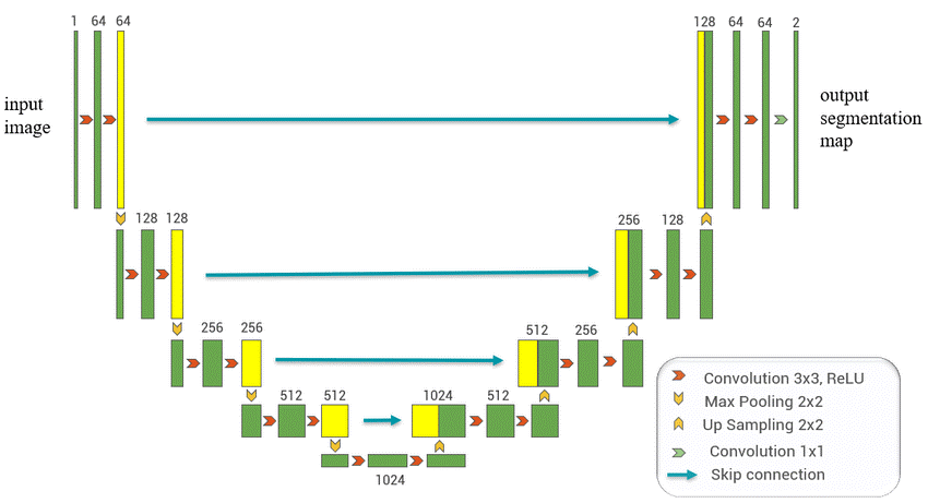
The whole architecture builds using a series of convolutional blocks where each block usually consists of two 3x3 convolutional layers. Create the building block of the U-Net model, the DoubleConv block, which consists of two convolutional layers with batch normalization and ReLU activation functions between them.
U-Net architecture is thoroughly divided into 5 steps:
- Encoder
- Decoder
- Bridge
- Skip Connection
- Output Segmentation Map
The basic terms used are
- in_c: input channels
- out_c: output channels
- features: image resolution
- kernel_size: height and width of the 2D convolution window
Step 1: Encoder
Encoder consists of four encoder blocks. The encoder network (contracting path) has half the spatial dimensions and double the number of filters (feature channels) at each encoder block.

for feature in features:
    self.downs.append(DoubleConv(in_c, feature))
    in_c = feature
Step 2: Decoder
Decoder consists of four decoder blocks. The decoder network (expanding path) doubles the spatial dimensions and half the number of feature channels at each decoder block.

for feature in reversed(features):
    self.ups.append(nn.ConvTranspose2d(feature*2,feature,kernel_size=2,stride=2))
    self.ups.append(DoubleConv(feature*2,feature)
Step 3: Bridge
The bridge in the U-Net architecture acts as a link between the encoder and decoder networks, facilitating the flow of information. It is composed of two convolutional layers, each with a size of 3x3.

self.bottleneck = DoubleConv(features[1], features[-1]*2)
Step 4: Skip Connections
One distinctive feature of the U-Net architecture is the skip connections that connect the contracting path with the corresponding layers in the expanding path. They serve as shortcut connections for gradients, facilitating precise localization and segmentation by effectively combining local and global contextual information.

    def forward(self,x):
        skip_connections = []
        for down in self.downs:
            x = down(x)
            skip_connections.append(x)
            x = self.pool(x)

        x = self.bottleneck(x)
        skip_connections = skip_connections[::-1]

        for ind in range(0,len(self.ups),2):
            x = self.ups[ind](x)
            skip_connection = skip_connections[ind//2]

            if x.shape != skip_connection.shape:
                x = tf.resize(x, size=skip_connection.shape[2:])

            concat_skip = torch.cat((skip_connection,x),dim=1)
            x = self.ups[ind+1](concat_skip)

        return self.final_conv(x)
Step 5: Output Segmentation Map
Finally, the decoder outputs the final segmentation map. This is achieved through a pixel-wise classification layer, typically a 1x1 convolutional layer with some activation.

self.final_conv = nn.Conv2d(features[0], out_c, kernel_size=1)
Data Preprocessing
Data preprocessing is a crucial step to prepare the dataset for training the U-Net model effectively. The following are the essential steps in data preprocessing:
- Data Collection
- Data Augmentation
- Normalization
- Resizing
- Data Splitting
Step 1: Data Collection
Create a labeled dataset with input images and ground truth masks, ensuring matching dimensions. Use the "Carvana" dataset and define functions like len() and get_item() in a separate class to build the custom dataset.
Initialization of Dataset class:
class Dataset(Dataset):
    #here transform is an optional parameter
    def __init__(self,image_dir,mask_dir,transform=None):
        self.image_dir = image_dir  #getting images path
        self.mask_dir = mask_dir    #getting masks path of corresponding images
        self.transform = transform  #data transformation on images & masks
        self.images = os.listdir(image_dir)   #getting filenames as list
Getting Size of dataset:
    #finding the number of images in the dataset
    def __len__(self):
        return len(self.images)
Accessing each image and mask for given index:
    #retrieve an image from the dataset based on the given index
    def __getitem__(self,index):
        #full path of image & mask
        img_path = os.path.join(self.image_dir,self.images[index])
        mask_path = os.path.join(self.mask_dir,self.images[index].replace(".jpg","_mask.gif"))

        #open an image in RGB mode & mask in Grayscale mode.
        image = np.array(Image.open(img_path).convert("RGB"))
        mask = np.array(Image.open(mask_path).convert("L"),dtype=np.float32)
        #convert masks from range [0, 255] to [0, 1]
        mask[mask == 255.0] = 1.0

        if self.transform is not None:    #if transformation is applied
            augs = self.transform(image=image,mask=mask)
            image = augs["image"]
            mask = augs["mask"]

        return image,mask
Step 2: Data Augmentation
To avoid overfitting for the dataset, apply data augmentation techniques such as rotation, flipping, and scaling to create additional training samples.
import albumentations as A
 A.Compose(
        [
            A.Rotate(limit=35, p=1.0),
            A.HorizontalFlip(p=0.5),
            A.VerticalFlip(p=0.1),
            ToTensorV2(), #converts input image or array to a pytorch tensor
        ],
          )
Step 3: Normalization
Normalize the pixel values of the input images to a common range (e.g., [0, 1] or [-1, 1]). Normalization improves convergence during training and prevents numerical instability.
A.Normalize(
        mean=[0.0, 0.0, 0.0],
        std=[1.0, 1.0, 1.0],
        max_pixel_value=255.0,
           ),
Step 4: Resizing
Resize the input images and masks to a uniform size compatible with the U-Net model. Commonly, square images are preferred to simplify the architecture.
A.Resize(
        height=IMAGE_HEIGHT,
        width=IMAGE_WIDTH
         ),
After performing data transformation on both the training and validation sets, the entire code appears as given below:
    #defining transformation of train images
    train_transform = A.Compose(
        [
            A.Resize(height=IMAGE_HEIGHT, width=IMAGE_WIDTH),
            A.Rotate(limit=35, p=1.0),
            A.HorizontalFlip(p=0.5),
            A.VerticalFlip(p=0.1),
            A.Normalize(
                mean=[0.0, 0.0, 0.0],
                std=[1.0, 1.0, 1.0],
                max_pixel_value=255.0,
            ),
            ToTensorV2(), #converts input image or array to a pytorch tensor
        ],
    )

    #defining transformation of validation images
    val_transform = A.Compose(
        [
            A.Resize(height=IMAGE_HEIGHT, width=IMAGE_WIDTH),
            A. Normalize(
                mean = [8.0, 0.0, 0.0],
                std = [1.0, 1.0, 1.0],
                max_pixel_value=255.0,
            ),
            ToTensorV2(),
        ],
    )
Step 5: Data Splitting
Divide the dataset into training, validation, and testing (if needed) sets. The training set is used for model optimization, the validation set for hyperparameter tuning, and the testing set to evaluate the final model's performance.
TRAIN_IMG_DIR = "train_images PATH"
TRAIN_MASK_DIR= "train_masks PATH"
VAL_IMG_DIR = "val_images PATH"
VAL_MASK_DIR = "val_masks PATH"
Model Training
Model training aims to build the best mathematical representation of the relationship between data and a target (supervised) or among the data itself (unsupervised). Model training is the process of feeding engineered data to a parametrized machine learning algorithm in order to output a model with optimal learned trainable parameters that minimize an objective function.
Step 1: Define Hyperparameters
Define hyperparameters for model training, including learning rate, device, batch size, epochs, data loading workers, image dimensions, pin memory, and load model option.
LEARNING_RATE = 1e-4
DEVICE = "cuda" if torch.cuda.is_available() else "cpu"
BATCH_SIZE= 16
NUM_EPOCHS = 1
NUM_WORKERS = 5
IMAGE_HEIGHT = 160
IMAGE_WIDTH = 240
PIN_MEMORY = True
LOAD_MODEL = True
Step 2: Load Data and Model Setup
Create the U-Net model instance. Define the loss function (Binary Cross Entropy with Logistic) and optimizer (Adam) for model training. Load the training and validation datasets using data loaders.
    model = UNet(in_c=3,out_c=1).to(DEVICE)  #U-Net model instance
    loss_fn = nn.BCEWithLogitsLoss()   #cross entropy loss
    optimizer = optim.Adam(model.parameters(), lr=LEARNING_RATE) #Adam  Optimizer

    train_loader, val_loader = get_loaders(
        TRAIN_IMG_DIR,
        TRAIN_MASK_DIR,
        VAL_IMG_DIR,
        VAL_MASK_DIR,
        BATCH_SIZE,
        train_transform,
        val_transform
    )
Step 3: Load Checkpoint
If LOAD_MODEL is set to True, load a previously saved model checkpoint for continuing training.
if LOAD_MODEL:
     load_checkpoint(
         torch.load("my_checkpoint.pth.tar PATH"),
         model
     )
It is optional in model training and requires load_checkpoint() and save_checkpoint() functions to work on. These functions loads the previous saved model and save the newly created model respectively.
#saving the models current state
def save_checkpoint(state, filename="my_checkpoint.pth.tar PATH"):
    print("=> Saving checkpoint")
    torch.save(state, filename)
Step 4: Define the Training Function
- Implement the training function for one iteration.
- Making the train samples into batches using "tqdm" loop library.
- Use a gradient scaler to handle mixed-precision training for better GPU memory usage.
#training function that is for one iteration
def train_fn(loader,model,optimizer,loss_fn,scaler):
    loop = tqdm(loader)       #tqdm library provides progress for iterations

    #batch_ind is index, data & target are tensors contained in current batch
    for batch_ind, (data, targets) in enumerate(loop):
        data = data.to(device=DEVICE)
        targets = targets.float().unsqueeze(1).to(device=DEVICE)

        #forward
        with torch.cuda.amp.autocast(): #enable automatic mixed-precision(amp)
            pred = model(data)
            loss = loss_fn(pred,targets)


     	#backward
        optimizer.zero_grad() #clears the gradients of all optimized parameters
        #scales loss value by scaler to handle mixed-precision training
        scaler.scale(loss).backward()
        #updates model parameters by performing optimization step
        scaler.step(optimizer)
        scaler.update()

        #update tqdm loop using loop variable with current loss value.
        loop.set_postfix(loss=loss.item())
Step 5: Training Loop
- Execute the training loop for the specified number of epochs.
- Save the model's state dictionary and checkpoint after each epoch.
- Finally, evaluate the model's accuracy.
def main():
    #defining transformation of train & validation images
    #load and setup model with loss function and optimizer
    #load_checkpoint

    scaler = torch.cuda.amp.GradScaler()

    #training model with the given number of epochs
    for epoch in range(NUM_EPOCHS):
        train_fn(train_loader,model,optimizer,loss_fn,scaler)

        #save the model in state_dict
        checkpoint = {
            "state_dict": model.state_dict(),
            "optimizer": optimizer.state_dict(),
        }
        save_checkpoint(checkpoint)

        #evaluation of trained model
        print("Epoch", epoch)
Step 6: Evaluation
To properly configure the model, certain parameters such as accuracy and dice score are essential. Subsequently, the generated images are stored in a designated folder. To conduct evaluations, the model is switched to evaluation mode before reverting back to the training mode.
For calculating accuracy of trained model:
def check_accuracy(loader,model,device="cuda"):
    num_correct = 0
    num_pixels = 0
    dice_score = 0
    model.eval() #model is set to evaluation mode
    with torch.no_grad():
        for x, y in loader:
            x = x.to(device)
            y = y.to(device).unsqueeze(1)

             #giving sigmoid activation function for model
            preds = torch.sigmoid(model(x))

             #setting threshold of predicting to 0.5
            preds = (preds > 0.5).float()

            num_correct += (preds == y).sum()
            num_pixels += torch.numel(preds)
            dice_score += (2*(preds*y).sum()) / ((preds + y).sum()+1e-8)

    print(f"Got {num_correct}/{num_pixels}
	with accuracy {num_correct/num_pixels*100:.2f}")

    print(f"Dice Score: {dice_score/len(loader)}")
    model.train() #model is setting back to training mode
MlFlow Tracking
MlFlow is an open-source platform to manage and track machine learning experiments. It helps in keeping track of parameters, metrics, and artifacts for reproducibility and collaboration. To integrate MlFlow with our U-Net model training, follow these steps:
Step 1: Install MlFlow and Necessary Libraries
Install mlflow with the following commands.
!pip install mlflow --quiet
!pip install pyngrok –quiet
Import requires libraries for model tracking using mlflow.
import mlflow
import mlflow.pytorch
from pyngrok import ngrok
Step 2: Set Up MlFlow Tracking
- Track all the parameters and metrics using autolog or defining explicitly.
- Terminate already running tunnels and MlFlow runs.
- Start a new run by logging the created model.
# creating model instance
model = UNet(in_c=3, out_c=1).to(DEVICE)

mlflow.autolog() #automatic logging of all params and metrics

ngrok.kill() # Terminate open tunnels if exist
mlflow.end_run() # Terminate already running runs if exist
#starting a new run
with mlflow.start_run() as run:
    #explicitly logging of required params and metrics if needed
    mlflow.pytorch.log_model(model, "models") #logging our model
Step 3: Run MlFlow UI
To track the model must run MlFlow UI in the background on port number 5000.
get_ipython().system_raw("mlflow ui --port 5000 &")
Step 4: Set Up ngrok Tunnel
- Set up a ngrok tunnel to expose the MlFlow Tracking UI to access it externally.
- Provide Auth token and then connect ngrok tunnel to port number 5000.
- Finally get URL of MlFlow Tracking UI.
# Setting the auth-token
NGROK_AUTH_TOKEN = "YOUR_NGROK_AUTH_TOKEN"
ngrok.set_auth_token(NGROK_AUTH_TOKEN)

# Open an HTTPs tunnel on port 5000
ngrok_tunnel = ngrok.connect(addr="5000", proto="http", bind_tls=True)
print("MLflow Tracking UI:", ngrok_tunnel.public_url)
Conclusion
Semantic segmentation with the U-Net model is a powerful technique for various computer vision tasks. By following this end-to-end guide, you can preprocess your data, train the U-Net model, and use MlFlow for experiment tracking, making your research or project more manageable, reproducible, and shareable. Happy experimenting😇😎😇!
References
https://towardsdatascience.com/unet-line-by-line-explanation-9b191c76baf5
https://paperswithcode.com/method/u-net
https://blog.paperspace.com/unet-architecture-image-segmentation/
https://mlflow.org/docs/latest/index.html
Also, Checkout
To know more about our company. Go through this https://aiensured.com/.
Want to check consequences due to an untested AI/ML model. Visit this https://blog.aiensured.com/disaster-due-to-untested-data-and-ml-model/.
Curious about various job opportunities in data science. Refer to this https://blog.aiensured.com/career-opportunities-in-data-science/.
To read more awesome articles. Check this https://blog.aiensured.com/.