Grad-CAM++: White Box Explainability for Image Classification
Grad-CAM ++ is one of the most reliable and widely used explainability techniques for CNN because of its lucidity and efficaciousness.
It is not a new fact that deep learning models offer tremendous benefits with impressive results in tasks like object detection, speech recognition, and machine translation to name a few. But one of the biggest challenges with deep learning is explaining to customers and regulators how the models get their answers. In many cases, we simply don’t know how the models generated their answers, even if we’re very confident in the answers themselves.
This is where the model Explainability which creates a saliency map for deep learning models for a given input, comes into the picture. The need for white box and black box explainability techniques for AI models is explained in detail in this article. There are different Model explainability techniques for the CNN image classification algorithm. In this article, we will look into the Grad CAM ++ model explainability technique.
Grad-CAM ++ is a Whitebox Machine Learning Explainability technique that produces the saliency map/heat map, which indicates exactly where the model is focusing on the image in the form of a saliency map but only if we know the internal aspects of the models.
Deep learning is a sub-area of machine learning. While both deep learning and machine learning falls under the category of artificial intelligence.
Whitebox machine learning approach explanations depend on the model's architecture and its internal aspect therefore the explanation given in the form of a saliency map by deep learning models is more accurate and gives better confidence in the explainer.
To know more about White box vs Black box explainability techniques (i.e. Model Specific & Model Agnostic Explainability) refer to this article.
GradCAM++ (Gradient weighted Class Activation Map Plus Plus)
Grad CAM++ has been an extension of methods CAM & Grad CAM, to provide better visual explanations of CNN image classification algorithm model predictions (when compared to Grad CAM), in terms of
- Better localization of objects
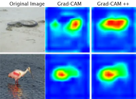
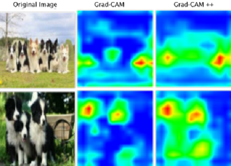
- Explaining occurrences of multiple objects of a class in a single image using saliency maps on deep learning models.
Grad CAM ++ uses the backpropagation and gradient descent method on the model for a given input to highlight class-relevant pixels by propagating the network output back to the input image space.
Grad CAM: Refer to this article for Grad CAM & Guided Grad CAM which are white box machine learning explainability techniques, both of these techniques also use backpropagation and gradient descent to produce a saliency map for deep learning models.
CAM, GRAD-CAM and Grad-CAM ++
- CAM method needs CNN image classification algorithm modification
- Grad CAM which is a white box machine learning explainability technique estimates the weight by dividing Z i.e. the size of the feature map. If the presence of the object area is small the weight becomes smaller, which means Grad CAM doesn’t give importance to such features/pixels.

- This will suppress activation maps with a comparatively lesser spatial footprint. And also the inability to identify multiple instances of objects.
GRAD CAM ++ solves the above issues
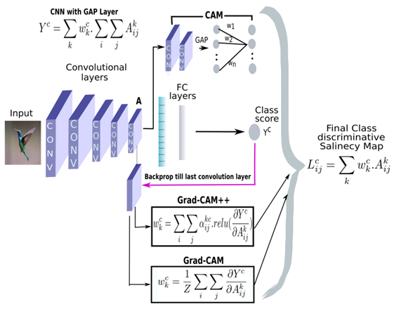
The difference between Grad CAM and Grad CAM ++ is in the weight calculation formula during backpropagation. Grad CAM ++ gives equal importance to all the pixels by multiplying α (which is calculated during backpropagation and gradient descent) in weight calculation.
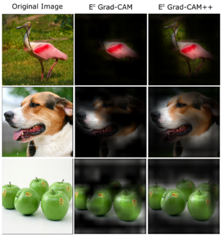
Let’s try to understand the Grad-CAM ++ visually
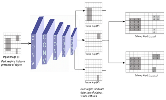
In the above figure 5 output, we can see that the Grad CAM saliency map for the deep learning model i.e., CNN is giving less pixel value(i.e., 0.26 & 0.13) for the features with less spatial footprint.
We are importing the TensorFlow "Functional API" model, where you start from Input, you chain layer calls to specify the model's forward pass, and finally, you create your model from inputs and outputs:
import numpy as np
import tensorflow as tf
from tensorflow.keras.models import load_model
from tensorflow.keras.preprocessing import image
from tensorflow.keras import Model
Now let’s see how Grad CAM ++ is giving equal importance to each pixel (i.e., occurrences of multiple objects) and object localization
- For a particular class ‘c’ and activation map ‘k’, Ak represents the visualization of the kth feature map, and the pixel-wise weight αkc at pixel position (i,j) can be calculated as: for occurrences of multiple objects in an image

where

Code for the above alpha formula.
Here we are getting the last convolution layer of the pre-trained model and also the output of the softmax layer (refer to fig 2) for applying during backpropagation and gradient descent. We are applying the power3 gradient as mentioned in the alpha formula. Then calculated the alpha and normalized it.
Yc refers to the output of the softmax layer.
Ak refers to the feature maps of the last convolution layer output.
img_tensor = np.expand_dims(img, axis=0)
conv_layer = model.get_layer(layer_name)
heatmap_model = Model([model.inputs], [conv_layer.output, model.output])

with tf.GradientTape() as gtape1:
    with tf.GradientTape() as gtape2:
        with tf.GradientTape() as gtape3:
            conv_output, predictions = heatmap_model(img_tensor)
            if category_id==None:
                category_id = np.argmax(predictions[0])
            if label_name:
                print(label_name[category_id])
            output = predictions[:, category_id]
            conv_first_grad = gtape3.gradient(output, conv_output)
        conv_second_grad = gtape2.gradient(conv_first_grad, conv_output)
    conv_third_grad = gtape1.gradient(conv_second_grad, conv_output)

global_sum = np.sum(conv_output, axis=(0, 1, 2))

alpha_num = conv_second_grad[0]
alpha_denom = conv_second_grad[0]*2.0 + conv_third_grad[0]*global_sum
alpha_denom = np.where(alpha_denom != 0.0, alpha_denom, 1e-10)

alphas = alpha_num/alpha_denom
alpha_normalization_constant = np.sum(alphas, axis=(0,1))
alphas /= alpha_normalization_constant

weights = np.maximum(conv_first_grad[0], 0.0)
deep_linearization_weights = np.sum(weights*alphas, axis=(0,1))
- Final localization of objects LGrad-CAM++ (similar to that of GradCAM)

Now we are applying our model's last convolution layer output to Grad-CAM ++ for visualizing the features, the model has considered giving specific output in the form of a saliency map by applying ReLU where negative gradients are suppressed when backpropagating through ReLU layers ( we are capturing pixels detected by neurons, not the ones that suppress neurons).
grad_CAM_map = np.sum(deep_linearization_weights*conv_output[0], axis=2)

heatmap = np.maximum(grad_CAM_map, 0)
max_heat = np.max(heatmap)
if max_heat == 0:
max_heat = 1e-10
heatmap /= max_heat
Conclusion
Grad-CAM++ white box machine learning explainability technique is a generalized class-discriminative approach for visual explanations of CNN-based architectures. We also discussed the formal derivation for the Grad-CAM++ method and showed how simple, yet effective the generalization of Grad-CAM is. The Grad-CAM++ method addresses the shortcomings of Grad-CAM, of not being able to detect multiple occurrences of the same class in an image and poor object localization. Grad-CAM ++ Explainability technique helps in building trust in the model prediction.
Do check out:
- One such magical product that offers explainability is AIEnsured by testAIng. Do check this link.