KNN Regressor and its fine-tuning
KNN ( K nearest neighbours) is a popular machine-learning model that is non-parametric and can be used for both categorical and continuous numerical data. KNN Classifier is used for categorical data while KNN Regressor is used for continuous data that predicts the numerical target based on similarity measure. It takes the average of the k nearest observations /neighbours and predicts the outcome.
KNN Regressor can also be used for imputing missing values which involves a few steps:
- Identifying the feature having the missing values and splitting the dataset into two with one having the feature containing missing values( target set ) and the other being complete( training set ).
- The data is preprocessed by using different scaling or normalising methods as having different scales in the data can affect the outcome of the KNN model. This will be covered in detail in this article.
- Create an instance of the KNN Regressor and fit it to the training set. Use the trained regressor model to predict the missing values in the target set.
The implementation of this model is simple. In this article, a health insurance dataset is used.
url = 'https://raw.githubusercontent.com/ChaithrikaRao/DataChime/master/insurance (2).csv'
df = pd.read_csv(url) #loading the dataset and reading into a variabledf
df.head(10) #printing the first 10 columns of the dataset
Here, the dataset is downloaded and the first 10 rows are printed.
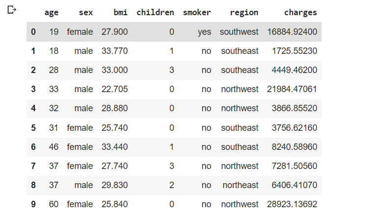
As shown there are eight columns with 3 categorical columns and the rest being continuous.
The variable ’charges’ is the target variable. Since the variable ‘region’ does not affect the outcome of the model and target variable, that column can be dropped.
df=df.drop(['region'],axis=1)
This dataset consists of more than 1338 rows and 7 columns (as one column is dropped). It is split into two parts of 1200 rows and the remaining. The first set of 1200 is used for training the regressor model.
df_1 = df[:1200] #spliting the data # the first 1000 -- df_part1 -- used for training the model
df_2 = df[1200:]
The KNN Regressor model works only for numerical data. So the categorical columns in the dataset are encoded such that they become compatible with the model. Here, the encoding is done using ‘get dummies’.
categorical_columns = ['sex', 'smoker']
df_1_encoded = pd.get_dummies(df_1, columns=categorical_columns,drop_first=True).rename(columns = {'sex_male': 'sex', 'smoker_yes': 'smoker'}, inplace = False)
Now this dataset ‘df_1’ is further divided into the set for training the model and target set.
X=df_1_encoded.drop('charges',axis=1) # dropping the charges column
y= df_1_encoded['charges'] #target variable
Before implementing the regression model, the data is preprocessed which includes processes like normalisation. It is done so that all the features will be of the same scale and contribute equally to the distance calculation. Preprocessing also ensures that the dataset will be consistent and properly formatted so that the imputation process is not affected. After this step, the dataset is further split into training data and testing data. To normalise all the values in the data, different techniques are used like z-score, log transformation, robust scaling, min-max scaler, etc…
Z-Score:
numerical_columns = ['age', 'bmi'] #identifying the numerical columns to apply z-score # Applying z-score transformation to numerical columns
X[numerical_columns] = X[numerical_columns].apply(zscore)
X_train, X_test, y_train, y_test = train_test_split(X, y, train_size=None, test_size=0.4, random_state=42) # Splitting the data into testing and training data
This adjusts the values such that the average of all the values in a column is nearly 0.
Min-Max scaler:
X_train, X_test, y_train, y_test = train_test_split(X_1, y_1, train_size=None, test_size=0.3, random_state=42)
scaler = MinMaxScaler() # Fit and transform the training set
X_train_scaled = scaler.fit_transform(X_train) # Transform the testing set
X_test_scaled = scaler.transform(X_test)
Here it is scaled after splitting the data into train and test sets.
Log-transformation:
X_log_transformed = np.log1p(X_1)
X_train, X_test, y_train, y_test = train_test_split(X_log_transformed, y_1, test_size=0.2, random_state=42)
Robust scaling:
X_train, X_test, y_train, y_test = train_test_split(X_1, y_1, train_size=None, test_size=0.3, random_state=42)
scaler = RobustScaler() # Fit and transform the training set
X_train_scaled = scaler.fit_transform(X_train) # Transform the testing set
X_test_scaled = scaler.transform(X_test)
The type of normalisation used and the properties of the dataset, both affect the accuracy of the regression model.
The model is then fit to the scaled dataset.
knn_model = KNeighborsRegressor(n_neighbors=5)
knn_model.fit(X_train, y_train)
y_pred = knn_model.predict(X_test)
print(("Train accuracy: ", knn_model.score(X_train, y_train)))
print(("Test accuracy: ", knn_model.score(X_test, y_test)))
This prints the testing and training accuracy of the model.
Among all the above transformations, log transformation gave the best result (before finetuning):
('Train accuracy: ', 0.8585893636184455) ('Test accuracy: ', 0.8129919043365657)
‘KNeighborsRegressor’ has many attributes like weight, n-neighbours, metric(distance), algorithm etc. These parameters play a major role in determining the accuracy and are often used to fine-tune the model. Some of the parameters we used are k value ( number of neighbours), weights, metric and algorithm.
There are several methods to find the optimal value for these parameters such that the accuracy of the model is high. One of them is the elbow method.
from sklearn.neighbors import KNeighborsRegressor
from sklearn.metrics import mean_squared_error
import numpy as np
error_rate = [] # Will take some time
for i in range(1, 40):
knn = KNeighborsRegressor(n_neighbors=i)
knn.fit(X_train, y_train)
pred_i = knn.predict(X_test)
error_rate.append(np.sqrt(mean_squared_error(y_test, pred_i)))
plt.figure(figsize=(10,6))
plt.plot(range(1,40),error_rate,color='blue', linestyle='dashed', marker='o',
markerfacecolor='red', markersize=10)
plt.title('Error Rate vs. K Value')
plt.xlabel('K')
plt.ylabel('Error Rate')
This generates a graph - Error rate vs K value.
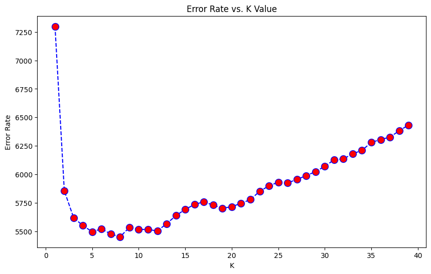
Here it is used after the log transformation of the data and similar graphs have been obtained for other methods too.
In this graph, we can see that the error rate is the least in the region between 5-10. We find the value of k for which the error rate levels off. This is the elbow point and is taken to be the optimal value. In this case, it is nearly around 10.
There are other methods to find the optimal values of the parameters like the ‘GridSearchCV’method. In this, we require a matrix of possible values of the parameters for which we will be using the range of k values in the above elbow method with a minimum error rate.
from sklearn.neighbors import KNeighborsRegressor
from sklearn.model_selection import GridSearchCV # 1. Define the parameter grid
param_grid_knn = {
'n_neighbors': [5,6,7,8,9,10,11,12,13,14],
'weights': ['uniform', 'distance'],
'p':[1,2],
'algorithm': ['ball_tree', 'kd_tree', 'brute', 'auto'],
'metric': ['minkowski', 'euclidean', 'manhattan', 'chebyshev']
} # 3. Create and fit the GridSearchCV
kNNModel_grid = GridSearchCV(estimator=KNeighborsRegressor(), param_grid=param_grid_knn, verbose=1, cv=10, n_jobs=-1)
kNNModel_grid.fit(X_train, y_train) # 4. Print the best estimator
print(kNNModel_grid.best_estimator_)
For log transformation:
Fitting 10 folds for each of 640 candidates, totalling 6400 fits KNeighborsRegressor(algorithm='brute', n_neighbors=12, p=1, weights='distance')
For z-score:
Fitting 10 folds for each of 640 candidates, totalling 6400 fits KNeighborsRegressor(algorithm='kd_tree', n_neighbors=7, p=1, weights='distance')
For min-max scaler:
Fitting 10 folds for each of 640 candidates, totalling 6400 fits KNeighborsRegressor(algorithm='brute', n_neighbors=12, p=1, weights='distance')
For robust scaling:
Fitting 10 folds for each of 640 candidates, totalling 6400 fits KNeighborsRegressor(algorithm='brute', n_neighbors=6)
The model is fit and the accuracies of each of the normalisation methods are checked and compared.
For z-score:
knn_model = KNeighborsRegressor(n_neighbors=8, weights='distance', algorithm = 'ball_tree',p=1, metric='minkowski')
knn_model.fit(X_train, y_train)
y_pred = knn_model.predict(X_test)
print(("Train accuracy: ", knn_model.score(X_train, y_train)))
print(("Test accuracy: ", knn_model.score(X_test, y_test)))
('Train accuracy: ', 1.0) ('Test accuracy: ', 0.7333146957761014)
For log transformation:
knn_model = KNeighborsRegressor(n_neighbors=12, weights='distance', algorithm = 'ball_tree',p=1, metric='euclidean')
knn_model.fit(X_train, y_train)
print(("Train accuracy: ", knn_model.score(X_train, y_train)))
print(("Test accuracy: ", knn_model.score(X_test, y_test)))
('Train accuracy: ', 1.0) ('Test accuracy: ', 0.8128859831793496)
For min-max scaler:
knn_model = KNeighborsRegressor(n_neighbors=10, weights='distance', algorithm = 'brute',p=2, metric='minkowski')
knn_model.fit(X_train_scaled, y_train)
y_pred = knn_model.predict(X_test_scaled)
print(("Train accuracy: ", knn_model.score(X_train_scaled, y_train)))
print(("Test accuracy: ", knn_model.score(X_test_scaled, y_test)))
('Train accuracy: ', 0.9999999999999846) ('Test accuracy: ', 0.8010932999140249)
For robust scaling:
knn_model = KNeighborsRegressor(n_neighbors=10, weights='distance', algorithm = 'brute',p=1, metric='minkowski')
knn_model.fit(X_train_scaled, y_train)
y_pred = knn_model.predict(X_test_scaled)
print(("Train accuracy: ", knn_model.score(X_train_scaled, y_train)))
print(("Test accuracy: ", knn_model.score(X_test_scaled, y_test)))
('Train accuracy: ', 1.0) ('Test accuracy: ', 0.8019309175709395)
The accuracy of the log-transformed data is the highest for both training and testing data. Therefore, this model is saved and used for further predictions.
In this article, we have seen how KNN Regressor can be useful for imputation and handling missing values.
Do Checkout:
To know more about such interesting topics visit this link.
Do visit our website to know more about our product.
References:
https://medium.com/analytics-vidhya/k-neighbors-regression-analysis-in-python-61532d56d8e4
https://www.saedsayad.com/k_nearest_neighbors_reg.htm
T Lalitha Gayathri