Optimizers in Neural Networks
These days we find AI everywhere, transforming the way we live and revolutionising industries. A fundamental concept of AI is the neural networks which play a significant role in powering intelligent systems. These networks mimic the structure of a human brain consisting of numerous interconnecting nodes processing vast amounts of data. But to maintain a decent accuracy and to be efficient they need optimizers. Optimizers are used to reduce the overall loss and improve the model's efficiency. This is done by adjusting the attributes of the network including weights and learning rates. Therefore, a suitable optimizer is chosen depending on the dataset and the model used for training the data.
Let us first understand the optimization process. The ultimate goal of the optimization process is to reduce the pre-defined loss function by adjusting the weights and other parameters. The loss function evaluates how well the model is predicting and it is calculated at every instance. The optimal value is found for each of the attributes of the network to yield the best performance. Gradient-based methods are dominant in this field, which calculate the gradient of the loss function concerning the parameters. However, there are other types of optimization methods that are used for different purposes.
Some of them are
- Gradient Descent
- Stochastic Gradient Descent
- Adam
- Adagrad
- Momentum
- RMSprop
Gradient Descent:
It is an iterative algorithm where it adjusts the parameters in opposite the direction to the gradient of the loss function. Gradually it reaches the minimum of the loss as it iterates. This works best for most purposes but at the same time, it is time-consuming and difficult to calculate the gradient if the dataset is huge and also it is not recommendable for nonconvex functions. It is mathematically shown as:
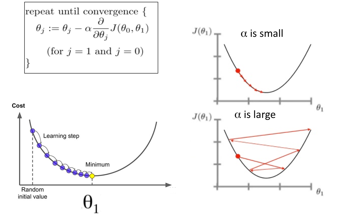
Fig: Source

Fig: Source
Stochastic Gradient Descent:
It is one of the variants of Gradient Descent where it randomly selects a batch of data. i.e. a subset of the training data instead of the entire dataset. Due to this, it requires higher iterations than gradient descent yet faster iterations. This increases the computational efficiency and also introduces randomness which helps to arrive at the global minima rather than getting stuck at a local minima.

Fig: Source

Fig: Source
Momentum:
This helps in accelerating the gradient descent when the curve is steeper in one direction than others by converging faster. It quickens the convergence, especially in noisy or shallow gradients and smooths out the process. This is done by adding a fraction of the previous update to the current update of the weights. It does not directly update the weights instead it uses a new variable ‘momentum term’ – a moving average of the gradients collecting the previous and current updates– which is used to update the weights.
Adagrad:
Adagrad is for Adaptive Gradient. Depending upon the gradient of the parameters, the learning rates of each of them are adjusted such that the higher gradient features have a slower learning rate and the lower gradient ones have a higher learning rate. That is, it adapts the learning rate of each parameter individually and removes the need for manual modification of the learning rates. This ensures that the process is fair for both dense and sparse datasets. This scaling of the learning rate helps to converge faster, accelerating the training of the network. But the only drawback of this model is that it reduces the learning rate aggressively and monotonically that at some point the rate may become extremely small. This is due to the accumulation of the squared gradients in the denominator.
RMSprop:
RMSprop stands for Root Mean Square Propagation. It is similar to the Adagrad optimizer in adapting the learning rates individually for the parameters. However, it improves upon Adagrad, using an exponentially weighted moving average of the squared gradients addressing the limitation of the Adagrad optimizer ensuring the learning rate doesn’t fall quickly. It also uses a decay factor that controls the influence of the previous gradients on the moving average and gives more weight to the recent gradients.

Fig: Source
Adam:
Adam stands for Adaptive Moment Estimation. It has a combined effect of both RMSprop and Momentum optimizations. It calculates a moving average of both the first and second moments of the gradient where one of them helps to move in the same direction even when there are smaller gradients and the other is used to adjust the learning rate for each of the parameters distinctly. It also maintains a bias correction factor that adjusts the moving averages which are biased towards zero at the beginning of the process by dividing them with a correction factor that accounts for the bias. But there are some drawbacks. It is computationally costly and tends to focus more on converging faster than on data points.
Do Checkout:
To know more about such interesting topics visit this link.
Do visit our website to know more about our product.
References:
https://ml-cheatsheet.readthedocs.io/en/latest/optimizers.html
https://dev.to/amananandrai/10-famous-machine-learning-optimizers-1e22
https://krishnaik.in/2022/03/28/understanding-all-optimizers-in-deep-learning/
https://keras.io/api/optimizers/
https://analyticsindiamag.com/guide-to-optimizers-for-machine-learning/
https://www.analyticsvidhya.com/blog/2021/10/a-comprehensive-guide-on-deep-learning-optimizers/
T Lalitha Gayathri