Sentiment Analysis Made Easy: Building, Deploying, and Tracking with Logistic Regression, Flask, and MLflow
In today's digital age, the explosion of text data on social media, product reviews, and online discussions has made sentiment analysis an essential tool for businesses and researchers alike. Sentiment analysis involves the use of Natural Language Processing (NLP) techniques to determine the underlying sentiment expressed in a piece of text, be it positive, negative, or neutral. Understanding sentiment can provide valuable insights into customer feedback, market trends, and public opinions.

In this article, we will embark on a journey to create a sentiment classification model using logistic regression, a simple yet powerful classification algorithm. We will explore how to preprocess the text data, extract meaningful features, and train the model to make accurate sentiment predictions. Once the model is ready, we will deploy it using Flask, a popular web framework, allowing users to interact with the sentiment classifier through a user-friendly web interface.
Additionally, we will leverage MLflow, an open-source platform for managing the machine learning lifecycle, to track the model's training process, hyperparameters, and performance metrics. MLflow will provide us with valuable insights into the model's performance, enabling us to make data-driven decisions and continuously improve the sentiment classifier.
Whether you're a data scientist looking to apply sentiment analysis in your projects or a developer seeking to integrate NLP capabilities into your applications, this article will serve as a comprehensive guide to building, deploying, and monitoring a sentiment classification model using logistic regression, Flask, and MLflow. So, let's dive in and unlock the power of sentiment analysis for various real-world applications!
Building the sentiment analysis model using Logistic regression :
Step 1: Data Collection
Before diving into building the sentiment classification model, we need a well-prepared dataset. The first step is to collect a labeled dataset for sentiment analysis. There are numerous sources available, such as online repositories or APIs, where you can find sentiment-labeled data.
For this sentiment analysis project, we obtained the dataset from Kaggle's "Sentiment140" dataset, a widely-used dataset for sentiment analysis tasks. The dataset contains 1.6 million tweets that are labeled with sentiments. Each tweet is associated with a sentiment label, where 0 represents a negative sentiment and 4 represents a positive sentiment.
The dataset is provided in CSV format and includes two main columns: "text": This column contains the text content of each tweet.
"sentiment": This column contains the corresponding sentiment label.
Step 2: Data Preprocessing
Before we can train a machine learning model, it is essential to preprocess the text data to make it suitable for analysis. The preprocessing steps involve transforming the raw text data into a clean and structured format. Let's outline the data preprocessing steps we will perform:
Lowercasing: We begin by converting all the text to lowercase using the ‘lower()’ method.
Removing URLs and Emojis: The regex pattern ‘urlPattern’ is used to match and replace all URLs in the tweet text with the word 'URL'. The emojis library is used to detect and replace ‘emojis’ with placeholders like 'EMOJIsmiley'.
Handling User Mentions: The regex pattern ‘userPattern’ is used to match and replace user mentions (e.g., @username) with the word 'USER'.
Removing Non-Alphabetic Characters: The regex pattern ‘alphaPattern’ is used to match and remove all non-alphabetic characters from the tweet text.
Reducing Consecutive Letters: The regex pattern ‘sequencePattern’ is used to match three or more consecutive letters and replace them with just two letters using ‘seqReplacePattern’.
Lemmatization: We use the ‘WordNetLemmatizer’ from NLTK to perform lemmatization on each word in the tweet. Lemmatization reduces words to their base form, ensuring consistency and reducing feature dimensionality.
def preprocess(textdata):
processedText = []

# Create Lemmatizer and Stemmer.
wordLemm = WordNetLemmatizer()

# Defining regex patterns.
urlPattern        = r"((http://)[^ ]*|(https://)[^ ]*|( www\.)[^ ]*)"
userPattern       = '@[^\s]+'
alphaPattern      = "[^a-zA-Z0-9]"
sequencePattern   = r"(.)\1\1+"
seqReplacePattern = r"\1\1"

for tweet in textdata:
    tweet = tweet.lower()

    # Replace all URls with 'URL'
    tweet = re.sub(urlPattern,' URL',tweet)
    # Replace all emojis.
    for emoji in emojis.keys():
        tweet = tweet.replace(emoji, "EMOJI" + emojis[emoji])
    # Replace @USERNAME to 'USER'.
    tweet = re.sub(userPattern,' USER', tweet)
    # Replace all non alphabets.
    tweet = re.sub(alphaPattern, " ", tweet)
    # Replace 3 or more consecutive letters by 2 letter.
    tweet = re.sub(sequencePattern, seqReplacePattern, tweet)

    tweetwords = ''
    for word in tweet.split():
        # Checking if the word is a stopword.
        #if word not in stopwordlist:
        if len(word)>1:
            # Lemmatizing the word.
            word = wordLemm.lemmatize(word)
            tweetwords += (word+' ')

    processedText.append(tweetwords)

return processedText
By completing these preprocessing steps, we transformed the raw tweet data into a structured format suitable for training our sentiment classification model.
Step 3: Exploratory Data Analysis (EDA)
To gain insights into the dataset's sentiments, we conducted Exploratory Data Analysis (EDA) using word clouds. We split the preprocessed data into negative and positive tweets. The word clouds visually represented the most frequent words in each category.
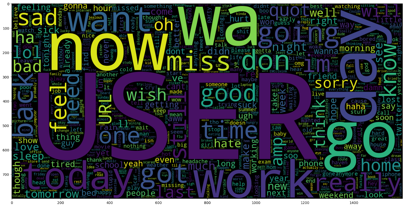
Word Cloud for Negative Tweets:
data_neg = processedtext[:800000]
plt.figure(figsize = (20,20))
wc = WordCloud(max_words = 1000 , width = 1600 , height = 800,
collocations=False).generate(" ".join(data_neg))
plt.imshow(wac)
We generated a word cloud for negative tweets by visualizing the most common words in the first 800,000 preprocessed entries. This allowed us to identify frequently occurring negative sentiment-related words.
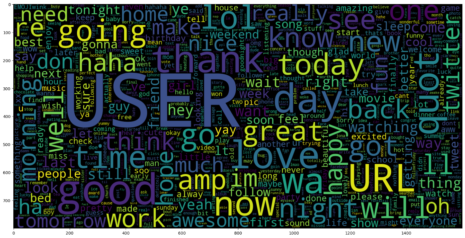
Word Cloud for Positive Tweets:
data_pos = processedtext[800000:]
wc = WordCloud(max_words = 1000 , width = 1600 , height = 800,
collocations=False).generate(" ".join(data_pos))
plt.figure(figsize = (20,20))
plt.imshow(wc)
Similarly, we created a word cloud for positive tweets by visualizing the most common words in the last 800,000 preprocessed entries. This provided insights into frequently occurring positive sentiment-related words. By analyzing these word clouds, we gained initial understanding of the dataset's characteristics and the common words associated with different sentiments.
Now we split the preprocessed text data and sentiment labels into training and testing sets using train_test_split from scikit-learn. The training set (X_train) consists of 95% of the data, while the testing set (X_test) contains the remaining 5%. We are now ready to proceed with feature extraction.
X_train, X_test, y_train, y_test = train_test_split(processedtext, sentiment,
test_size = 0.04, random_state = 0)
print(f'Data Split done.')
Step 4: Feature Extraction using TF-IDF
In this step, we will extract numerical features from the preprocessed text data using the TF-IDF (Term Frequency-Inverse Document Frequency) representation to extract numerical features from the preprocessed text data. The TfidfVectorizer from scikit-learn was used with an n-gram range of (1, 2) to consider both unigrams and bigrams. We limited the number of features to 500,000 for manageable dimensions.
vectoriser = TfidfVectorizer(ngram_range=(1,2), max_features=450000)
vectoriser.fit(X_train)
X_train = vectoriser.transform(X_train)
X_test = vectoriser.transform(X_test)
vectorizer.fit(X_train): We fitted the vectorizer on the training data to learn the vocabulary and IDF values.
X_train = vectorizer.transform(X_train): The training data was transformed into TF-IDF feature vectors.
X_test = vectorizer.transform(X_test): The testing data was transformed using the learned vocabulary and IDF values to ensure consistency in feature representation.
With feature extraction complete, we can now move on to train the sentiment classification model using logistic regression.
Step 4: Model training using Logistic Regression
Now that we have extracted the TF-IDF features from the preprocessed text data, we are ready to train our sentiment classification model. For this task, we will use logistic regression, a widely-used algorithm for binary classification tasks. Logistic regression works by finding the optimal weights for each feature, and this process is guided by minimizing the classification error on the training data.The goal of our model is to accurately predict whether a given tweet expresses a positive or negative sentiment.
LRmodel = LogisticRegression(C = 3, max_iter = 7000, n_jobs=-1)
LRmodel.fit(X_train, y_train)
model_Evaluate(LRmodel)
In the code above, we use LogisticRegression from scikit-learn to create an instance of the logistic regression model. We then train the model by calling the fit method and passing in the TF-IDF feature vectors ‘X_train’ and corresponding sentiment labels ‘y_train’. The model learns to map the numerical features to the sentiment labels during the training process.
Next, we will proceed to evaluate the performance of our trained sentiment classification model on the testing data.
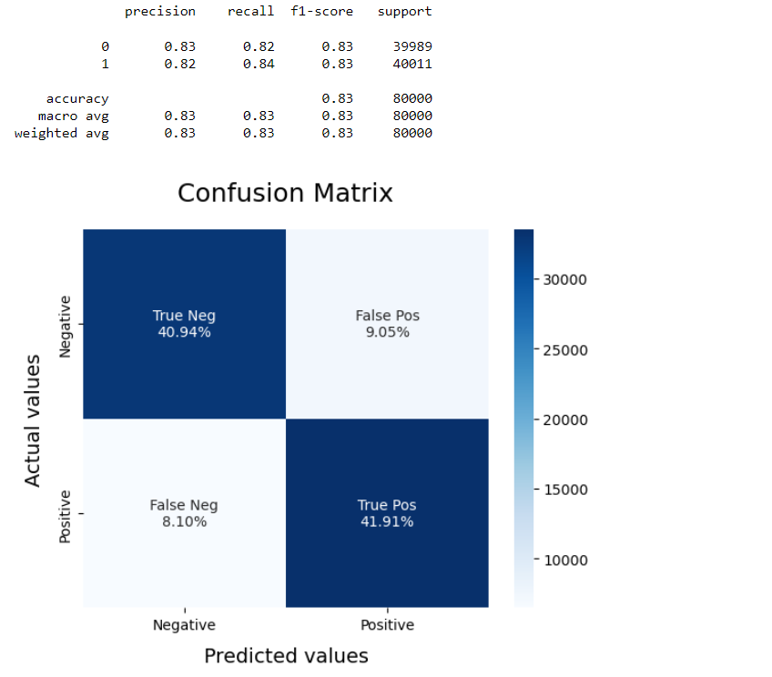
Step 6: Model Evaluation - Confusion Matrix and Classification Report
To further evaluate the performance of our sentiment classification model, we will implement a function called ‘model_Evaluate’. This function will provide valuable insights into the model's performance through a confusion matrix and a classification report.
def model_Evaluate(model):
# Predict values for Test dataset
y_pred = model.predict(X_test)

# Print the evaluation metrics for the dataset.
print(classification_report(y_test, y_pred))

# Compute and plot the Confusion matrix
cf_matrix = confusion_matrix(y_test, y_pred)

categories  = ['Negative','Positive']
group_names = ['True Neg','False Pos', 'False Neg','True Pos']
group_percentages = ['{0:.2%}'.format(value) for value in   cf_matrix.flatten() / np.sum(cf_matrix)]

labels = [f'{v1}\n{v2}' for v1, v2 in zip(group_names,group_percentages)]
labels = np.asarray(labels).reshape(2,2)

sns.heatmap(cf_matrix, annot = labels, cmap = 'Blues',fmt = '',
            xticklabels = categories, yticklabels = categories)

plt.xlabel("Predicted values", fontdict = {'size':14}, labelpad = 10)
plt.ylabel("Actual values"   , fontdict = {'size':14}, labelpad = 10)
plt.title ("Confusion Matrix", fontdict = {'size':18}, pad = 20)
In the code above, we define the ‘model_Evaluate’ function that takes the trained model as input. The function uses the ‘model’ to predict sentiment labels for the testing dataset (‘X_test’). It then prints a classification report, providing metrics such as precision, recall, F1-score, and support for both negative and positive sentiments.
The confusion matrix is also computed and visualized using the seaborn library. The confusion matrix helps us understand how well the model is predicting true positives, true negatives, false positives, and false negatives. The heatmap displays these values with their corresponding percentages for a clear understanding of the model's performance.
By using the ‘model_Evaluate’ function, we can easily assess the strengths and weaknesses of our sentiment classification model.
In the next section, we will proceed with deploying our sentiment classifier using Flask, creating a user-friendly web interface for sentiment analysis.
Step 5: Deployment with Flask :
Now that we have trained and evaluated our sentiment classification model, it's time to deploy it as a user-friendly web application using Flask. Flask is a lightweight and easy-to-use web framework in Python that enables us to create web applications quickly.
Deploying Sentiment Analysis Model using Flask for Real-time Sentiment Classification
Now we will explore how to deploy a sentiment analysis model using Flask, a lightweight web framework in Python. By deploying the model as a web application, users can interact with it in real-time, entering their own text and receiving sentiment predictions instantly. This deployment enables businesses to make data-driven decisions, analyze customer feedback, and monitor public sentiment about their products or services.
Step 1: Setting up Flask and Loading the Model
With the above sentiment analysis model, we set up a Flask web application. Flask allows us to create a user-friendly interface where users can interact with the model. We load the trained model and the TF-IDF vectorizer into the Flask app so that they can be accessed during the prediction process.
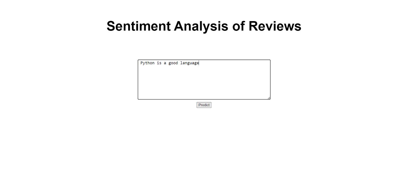
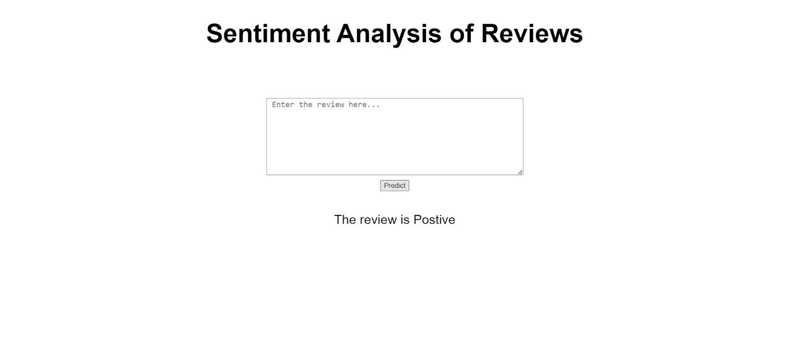
Step 3: Creating the User Interface (UI)
In this step, we design the user interface (UI) of the web application. We create an HTML template that includes a text input field where users can enter their text for sentiment analysis. Additionally, we add a button to trigger the prediction process and display the results.
<link
  rel="stylesheet"
  href="https://cdnjs.cloudflare.com/ajax/libs/font-awesome/4.7.0/css/font-awesome.min.css"
/>
<style>
  html {
    height: 100%;
  }

  body {
    height: 100%;
    font-family: Arial;
    margin: 0;
  }

  form {
    display: flex;
    align-items: center;
    flex-direction: column;
    justify-content: center;
  }

  form textarea {
    width: 500px;
    height: 150px;
    border-radius: 3px;
    padding: 2px 10px;
    box-sizing: border-box;
    min-width: 300px;
    margin-top: 29px;
    margin-bottom : 10px;
    font-size: 16px;
  }

  .container {
    height: 100%;
  }
  .header {
    height: 124px;
    margin-top: 0;
    padding: 36px;
    text-align: center;
    font-size: 25px;
  }


  .predict {
    margin-top: 42px;
    font-size: 25px;
    text-align: center;
  }


</style>
Sentiment Analysis of Reviews
Step 4: Sentiment Prediction with Flask
Once the user enters text and clicks the prediction button, Flask processes the input through the pre-processing steps, transforms it using the TF-IDF vectorizer, and feeds it into the trained logistic regression model. The model then predicts the sentiment label, which is displayed to the user on the web page.
import numpy as np
from flask import Flask, request, render_template
import joblib
app = Flask(name)
model = joblib.load(open('model.pkl', 'rb'))
cv = joblib.load(open('v.pkl', 'rb'))
@app.route('/')
def home():
return render_template('index.html')
@app.route('/predict', methods=['POST'])
def predict():
if request.method == 'POST':
    text = request.form['Review']
    data = [text]
    vectorizer = cv.transform(data)
    prediction = model.predict(vectorizer)
if prediction:
    return render_template('index.html', prediction_text='The review is Postive')
else:
    return render_template('index.html', prediction_text='The review is Negative.')
if name == "main":
app.run(debug=True)
At last run python app.py in command prompt

Now open http://127.0.0.1:5000 link in the chrome browser and enter test texts in the html page we built above , and check whether the sentiment predictions are accurate.
By deploying our sentiment analysis model using Flask, we have created a web application that enables real-time sentiment classification. Businesses and individuals can use this tool to understand public opinion, analyze customer feedback, and make data-driven decisions.This deployment showcases the power of NLP and demonstrates how we can make machine learning models accessible to a broader audience. As NLP technology continues to advance, deploying such applications will play an increasingly vital role in various industries, enhancing decision-making processes and gaining valuable insights from textual data.
MLflow Integration for Experiment Tracking
Now that we have deployed our sentiment analysis model using Flask, let's integrate MLflow to track our machine learning experiments automatically. MLflow provides a simple and efficient way to log and organize experiments, making it easier to compare different model versions and configurations.
Setting up MLflow
Make sure you have MLflow installed. If not, you can install it using pip:
At the beginning of our Python script (app.py), import MLflow and enable auto logging:
By adding just these two lines of code, MLflow will automatically track the parameters, metrics, and artifacts of our machine learning experiments.
Tracking Experiments
MLflow will automatically log the following information during our model training and evaluation:
- Parameters: MLflow logs all the parameters used in our script, including hyperparameters and other configuration settings.
- Metrics: MLflow tracks various metrics, such as accuracy, precision, recall, F1 score, etc., allowing us to compare different model versions easily.
- Artifacts: MLflow can log artifacts such as images, plots, and any other files generated during the model development process. In our case, we can log the word cloud images, the classification report, and the confusion matrix.
- Saving Model and Vectorizer as Artifacts :
To take advantage of MLflow's artifact logging, we can save the trained model and vectorizer as artifacts during deployment.
python Copy code import joblib # Save the model and vectorizer as artifacts mlflow.log_artifact("model.pkl") mlflow.log_artifact("vectorizer.pkl")
By using MLflow's artifact logging, we efficiently store our trained model and its associated artifacts. This allows us to easily retrieve the model and vectorizer for later use or to deploy the model in a different environment.
Tracking the Experiment:
With MLflow enabled, the model training and deployment process automatically becomes an experiment. MLflow will create a new experiment run each time we run the app.py script. We can view and compare these experiment runs using the MLflow UI.
To start the MLflow UI and view the experiments, open a new terminal or command prompt, navigate to the project directory, and run the following command: bash Copy code mlflow ui
The MLflow UI will be accessible at http://localhost:5000 by default. Here, you can see the logged parameters, metrics, and artifacts for each experiment run.
By integrating MLflow into our sentiment analysis application, we can easily track our model's performance and configurations, making it easier to manage and iterate on our machine learning projects.
In this article, we explored the process of building, deploying, and tracking a sentiment analysis model using logistic regression, Flask, and MLflow. We started by preparing the data and training the model with logistic regression. After that, we deployed the model using Flask, creating a user-friendly web application for sentiment analysis.
To enhance our model development process, we integrated MLflow for experiment tracking. MLflow automatically logged the model's parameters, metrics, and artifacts, making it easier to compare different versions of the model and manage experiments efficiently.
With MLflow, we saved the trained model and vectorizer as artifacts, allowing us to retrieve and reuse them later for deployment in different environments. This simplified the process of managing machine learning projects.
By combining logistic regression, Flask, and MLflow, we created a powerful sentiment analysis application that can be deployed and tracked with ease. This workflow enables efficient development and deployment of machine learning models for real-world applications.Happy coding and exploring the world of machine learning!....
References:
- https://towardsdatascience.com/sentiment-analysis-using-logistic-regression-and-naive-bayes-16b806eb4c4b
- https://www.freecodecamp.org/news/how-to-build-a-web-application-using-flask-and-deploy-it-to-the-cloud-3551c985e492/
- https://mlflow.org/docs/latest/index.html
Written by - Manohar Pali