SHAP Feature Importance in Audio Classification

Audio Classification is one of the most widely used applications nowadays and a lot of research has been done on classifying audio using different kinds of features and neural network architectures. Some real-world applications of this is Speaker Recognition, Music Genre Classification, and Bird Sound Classification.
The most commonly used features in audio are Spectrograms/Mel-spectrograms and state-of-the-art MFCCs. In this blog, we will learn about Audio Classification using MFCCs features and most importantly we will learn about Feature importance using SHAP.
Why SHAP Feature Importance?
SHAP feature importance not only tells us the most important and influential feature in making predictions but it also tells us which feature affects more for each class label.
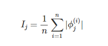
The idea behind SHAP feature importance is simple: Features with large absolute Shapley values are important. Since we want global importance, we average the absolute Shapley values per feature across the data.
Why SHAP over LIME?
LIME (Local Interpretable Model-agnostic Explanations) is another popular framework for feature importance analysis.
A long-standing and well-understood economic theory that guarantees the SHAP predictions are fairly distributed among the features whereas LIME does not guarantee this.
SHAP results provide an easy-to-read global interpretation method based on aggregations of Shapley values and a local view of the model predictions, whereas LIME only offers local interpretations.
The idea behind SHAP feature importance is simple: Features with large absolute Shapley values are important.
Since we want global importance, we average the absolute Shapley values per feature across the data. We sort the features by decreasing importance and plot them.
Let's get started with the implementation part...
We are importing the packages of pandas, librosa, layers for network and optimizers.
import librosa
import numpy as np
import matplotlib.pyplot as plt
import librosa.display
import pandas as pd
from sklearn.preprocessing import LabelEncoder
from sklearn.model_selection import train_test_split
from tensorflow.keras.utils import to_categorical
from tensorflow.keras.models import Sequential, load_model
from tensorflow.keras.layers import Dense, Dropout, Activation, Flatten, Reshape
from tensorflow.keras.layers import Convolution2D, Conv2D, MaxPooling2D, GlobalAveragePooling2D, LSTM, TimeDistributed
from tensorflow.keras.optimizers import Adam
from tensorflow.keras.callbacks import ModelCheckpoint
Data Loading and Feature Engineering step : We are loading the data using librosa package.
Librosa will help us in feature engineering by normalizing and Pre-emphasizing audio data. And in further steps, we will be doing padding in the data to make the size of all audio samples the same.
for directory in sub_dirs:
        audio_path = os.path.join(os.path.abspath(audio_dataset_path), str(directory) + '/')
        print(audio_path)
        files_count = 0
        for file in glob.glob(audio_path + "*.wav"):
            files_count = files_count + 1
            try:
                label = directory
                #Loading and normalisation
                audio, sample_rate = librosa.load(file, res_type='kaiser_fast')
                # Pre-emphasising audio data
                data = librosa.effects.preemphasis(audio)
                sr = sample_rate
                extracted_features.append([data, label])
            except:
                print('Audio file corrupted. Skipping one audio file')
                continue
        samples.append(files_count)

extracted_features_df = pd.DataFrame(extracted_features, columns=['feature', 'class'])
Converting the loaded extracted features into features variable and corresponding target variable then splitting the data.
X = np.array(extracted_features_df['feature'])
y = np.array(extracted_features_df['class'].tolist())
le = LabelEncoder()
yy = to_categorical(le.fit_transform(y))
x_train, x_test, y_train, y_test = train_test_split(X, yy, test_size=0.2, random_state=42)
Doing padding to the feature variables as in to make all samples of same length to pass on to the model.
def feature_extraction(audio, sr, max_pad_len):
    mfccs = librosa.feature.mfcc(y=audio, sr=sr, n_mfcc=40)
    print(mfccs)
    print(mfccs.shape)
    if (max_pad_len > mfccs.shape[1]):
        pad_width = max_pad_len - mfccs.shape[1]
        mfccs = np.pad(mfccs, pad_width=((0, 0), (0, pad_width)), mode='constant')
    else:
        mfccs = mfccs[:, :max_pad_len]
    return mfccs

final_x_train = []
for i in range(0, len(x_train)):
    audio = np.roll(x_train[i], int(sr / 10))  # Data Augmentation (time shifting)
    mfccs = feature_extraction(audio, sr, max_pad_len)
    final_x_train.append(mfccs)

x_train = np.array(final_x_train)

final_x_test = []
for i in range(0, len(x_test)):
    mfccs = feature_extraction(x_test[i], sr, max_pad_len)
    final_x_test.append(mfccs)

x_test = np.array(final_x_test)
Now, as we have got our data, now it's time for training the model, so we will reshape our data into a specific format according to TensorFlow model.
num_rows = 40
num_columns = 44
num_channels = 1
max_pad_len = 44

x_train = x_train.reshape(x_train.shape[0], num_rows, num_columns, num_channels)
x_test = x_test.reshape(x_test.shape[0], num_rows, num_columns, num_channels)
model architecture and training...
from tensorflow.keras.regularizers import l2
factor =  0.0001

model = Sequential()

model.add(Conv2D(filters=64, kernel_size=2,input_shape=(num_rows, num_columns, num_channels), activation='relu'))
model.add(MaxPooling2D(pool_size=2, padding='same'))
model.add(Dropout(0.2))

model.add(Conv2D(filters=128, kernel_size=2, kernel_regularizer=l2(factor), activation='relu'))
model.add(MaxPooling2D(pool_size=2, padding='same'))
model.add(Dropout(0.2))

model.add(Conv2D(filters=128, kernel_size=2,kernel_regularizer=l2(factor), activation='relu'))
model.add(MaxPooling2D(pool_size=2, padding='same'))
model.add(Dropout(0.2))

model.add(Conv2D(filters=256, kernel_size=2, activation='relu'))
model.add(MaxPooling2D(pool_size=2, padding='same'))
model.add(Dropout(0.2))

model.add(GlobalAveragePooling2D())

model.add(Reshape((4,64)))
model.add(LSTM(64, return_sequences=True))
model.add(Dropout(0.2))

model.add(Flatten())
model.add(Dense(units=64, activation='relu'))
model.add(Dropout(0.2))

model.add(Dense(num_labels, activation='softmax'))

model.compile(loss='categorical_crossentropy', metrics=['accuracy'], optimizer='adam')

checkpointer = ModelCheckpoint(filepath=model_save_path,
                               verbose=1, save_best_only=True)
start = datetime.now()

history = model.fit(x_train, y_train, batch_size=128, epochs=50, validation_data=(x_test, y_test), callbacks=[checkpointer], verbose=1)
Now we will install the SHAP using the pip command and after converting the data from 2D to 1D array by averaging the rows, then using SHAP kernel explainer to get the summary plot.
explainer = shap.KernelExplainer(pred_fn_shap_ale, X[0:10])
shap_values = explainer.shap_values(X, nsamples=10)
shap.summary_plot(shap_values, X, show=False, class_names=class_names)
The following figure shows the SHAP feature importance for the audio classification model trained on the music dataset.
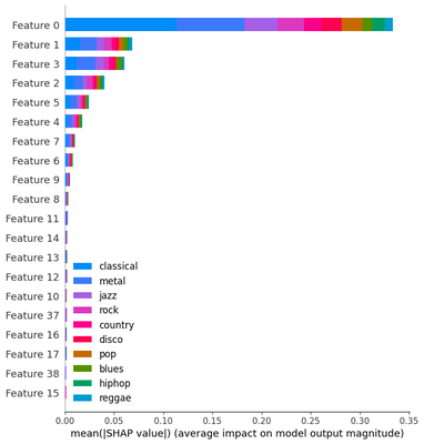
In the plot, we can see that the top 20 MFCCs feature has been shown in decreasing order of their importance. And we can also see from the color bar which feature influences a particular class more than the other.
In this way, SHAP helps in looking at feature importance at the class level as well as at the data level and makes model interpretation easy.
References :