End to End TEXT CLASSIFICATION

Text classification is a natural language processing (NLP) task that involves automatically categorizing or assigning predefined labels to text documents based on their content. The goal is to develop a machine learning model that can learn from labeled training data and accurately predict the class or category of unseen or new text data.

Text classification has various applications, such as sentiment analysis, spam detection, topic categorization, language identification, and intent recognition. It can be used in industries like e-commerce, customer service, social media monitoring, content filtering, and many others.

DATA PREPROCESSING:

Word Embedding:Word2Vec

Word2vec is a technique for natural language processing (NLP) that uses a neural network model to learn word associations from a large corpus of text. It produces a vector space, typically of several hundred dimensions, with each unique word in the corpus being assigned a corresponding vector in the space. The vectors capture the semantic and syntactic qualities of words, such that similar words have similar vectors².

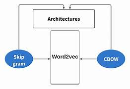
Word2vec is not a single algorithm, but a family of model architectures and optimizations that can be used to learn word embeddings. The two main architectures are *continuous bag-of-words (CBOW)* and *continuous skip-gram*. CBOW predicts a word given the surrounding context, while skip-gram predicts the context given a word¹. Both architectures use a shallow, two-layer neural network that is trained to reconstruct linguistic contexts of words

The main idea behind Word2Vec is to represent words as dense, continuous vectors in a high-dimensional space, where words with similar meanings or contexts are located closer to each other. These vector representations allow algorithms to process and understand the meaning of words in a numerical format, which is more convenient for machine learning models.

The key idea behind Word2Vec is to learn word embeddings by training a neural network on a large corpus of text. There are two main variations of the Word2Vec model: Continuous Bag of Words (CBOW) and Skip-gram.

Continuous Bag of Words (CBOW): In the CBOW model, the goal is to predict a target word based on its surrounding context words. The context words are used as input, and the target word is the output. The CBOW model learns to predict the target word by optimizing the parameters of the neural network using techniques like backpropagation and gradient descent.

Skip-gram: The skip-gram model is the inverse of CBOW. It takes a target word as input and tries to predict the context words around it. The skip-gram model also learns by optimizing the neural network parameters through backpropagation and gradient descent.

Both CBOW and skip-gram models create dense vector representations for words, where each dimension of the vector captures certain semantic or syntactic properties of the word.

The CBOW model aims to predict a target word based on its context, which consists of the surrounding words within a fixed window size. In contrast, the skip-gram model predicts the context words given a target word. Both models are trained using a technique called negative sampling, where a small subset of the words that do not appear in the context are sampled as negative examples during training.

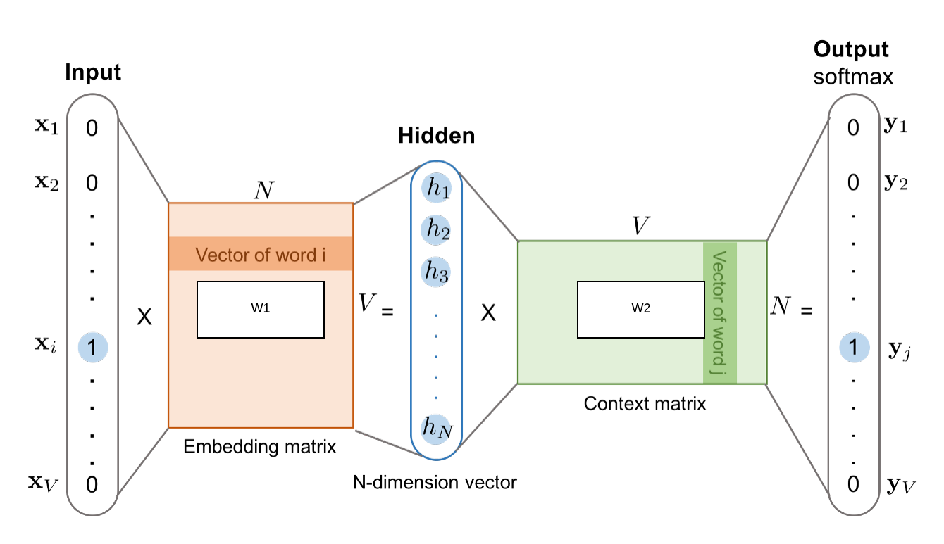
Once trained, the neural network model produces word embeddings as the weights of the hidden layer. These embeddings encode semantic and syntactic relationships between words, such that similar words have similar vector representations. For example, the vector representations of "king" and "queen" are expected to be closer to each other than to the vector representation of "dog."

Uses:

1.Semantic Similarity: Word2Vec embeddings can be used to measure the semantic similarity between words or sentences. By computing the cosine similarity between the vector representations of two words or sentences, you can determine their semantic relatedness. This can be applied in tasks like information retrieval, question answering, and recommender systems.

2.Sentiment Analysis: Word2Vec embeddings can be incorporated into sentiment analysis models to capture the sentiment or emotional content of text. The embeddings provide a representation of words that encapsulates their semantic meaning, allowing the model to understand the sentiment expressed in a given text.

3.Named Entity Recognition (NER): NER models aim to identify and classify named entities in text, such as names of people, organizations, locations, and more. Word2Vec embeddings can be used as features in NER models to capture the context and semantic information surrounding named entities, improving their recognition accuracy.

4.Text Classification: Word2Vec embeddings can be utilized as input features in text classification models such as convolutional neural networks (CNNs) or recurrent neural networks (RNNs). By representing words as vectors, the model can capture the contextual information and learn the relationships between words, leading to improved classification Performance.

5.Machine Translation: Word2Vec embeddings have been employed in machine translation models to improve translation quality. The embeddings can aid in capturing the semantic meaning of words in different languages and facilitate more accurate translation between them.

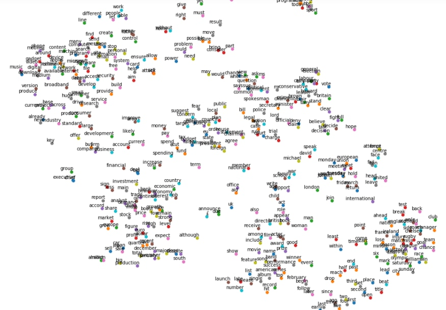
Representation of text into vectors in 2-D form

Disadvantages:

1.Lack of contextual information

2.Out-of-vocabulary words

3.Difficulty with rare words and phrases

4.Inability to handle polysemy and homonymy

5.Fixed-size word representations

6.Training data sensitivity

7.Computational requirements

Functions used in Word2Vec:

1.Tokenization

2.Context Window

3.One-Hot Encoding

4.Neural Network Architecture

5.Softmax Function

6.Negative Sampling

7.Gradient Descent Optimization

Example:

A portion in a sentence:

…like Data science…

“Like “ is the context word for both data and science.

“Data” and “Science” are the main words.

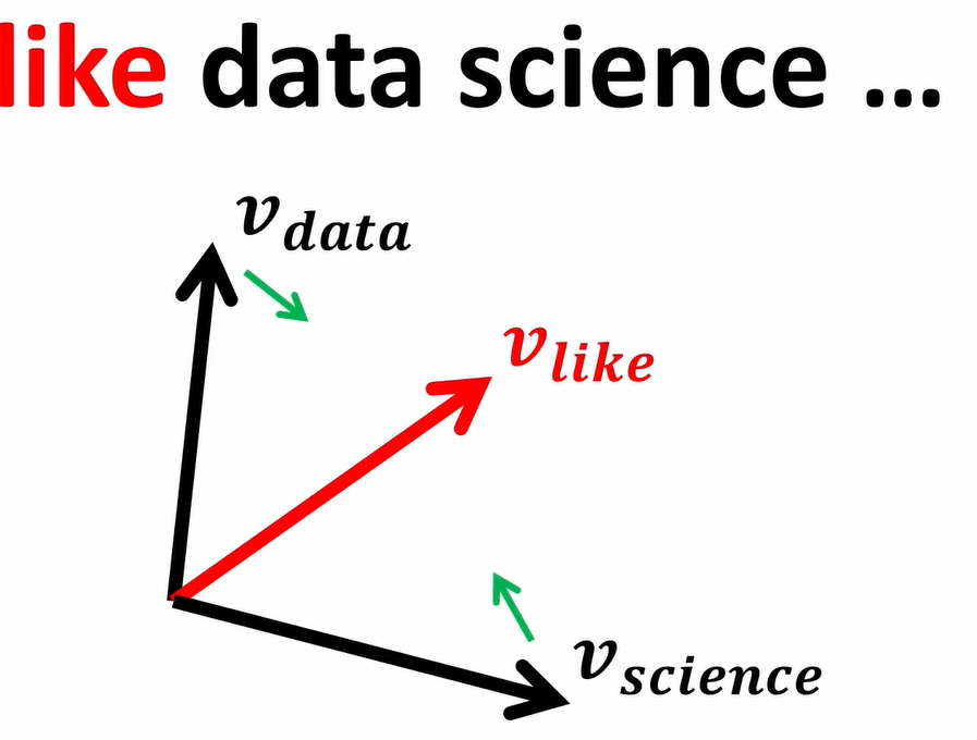
In this process the main vectors move close towards the context vector “like”.

In the next iteration,the two main vectors moves even close to the common context vector.

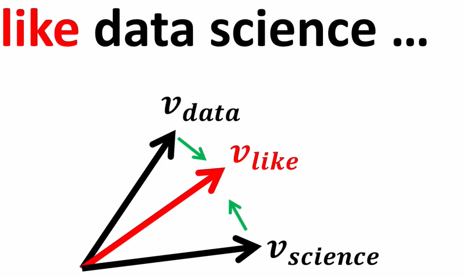
So,that will become:

At the end of the algorithm we will discard the context vector and we will end up with only two main embeddings i.e.,data and science.

Code:

Importing libraries

import pandas as pd
import nltk
import re
from nltk.corpus import stopwords
from nltk.stem.porter import PorterStemmer
from sklearn.feature_extraction.text import CountVectorizer
from sklearn.model_selection import train_test_split
from sklearn.naive_bayes import MultinomialNB
import joblib

Loading the dataset

df = pd.read_csv('Restaurant_Reviews.tsv', delimiter='\t')
corpus = []

import nltk
nltk.download('stopwords')

Looping till 1000 because the number of rows are 1000

for i in range(0, 1000):
# Removing the special character from the reviews and replacing it with space character
review = re.sub(pattern='[^a-zA-Z]', repl=' ', string=df['Review'][i])
# Converting the review into lower case character
review = review.lower()
# Tokenizing the review by words
review_words = review.split()
# Removing the stop words using nltk stopwords
review_words = [word for word in review_words if not word in set(
stopwords.words('english'))]
# Stemming the words
ps = PorterStemmer()
review = [ps.stem(word) for word in review_words]
# Joining the stemmed words
review = ' '.join(review)
# Creating a corpus
corpus.append(review)

Converting into lowercase:

The lowercase_texts list is created by converting each word in each sentence of common_texts to lowercase using a list comprehension. This ensures that all words in the training data are in lowercase before training the Word2Vec model.

Tokenization:

Tokenization is the process of breaking down a text or a sequence of characters into smaller units called tokens. These tokens can be words, subwords, or even characters, depending on the level of granularity needed for a particular task. Tokenization is a fundamental step in natural language processing (NLP) and is often a crucial preprocessing step before further analysis.

Removing stopwords:

Stopwords are common words that often appear in a language but typically do not carry significant meaning or value in certain NLP tasks, such as text classification or sentiment analysis. Examples of stopwords in English include "the," "is," "and," "of," etc.

Removing stopwords can help reduce the dimensionality of the data and focus on the more important words or tokens. Popular Python libraries like NLTK and spaCy provide built-in sets of stopwords that you can use to filter out these words from your text data.

Stemming:

Stemming is a natural language processing (NLP) technique used to reduce words to their base or root form, called the "stem." The purpose of stemming is to normalize words, so different variations of the same root word are treated as the same word. This process helps in reducing the vocabulary size, simplifying text analysis, and improving the efficiency of information retrieval and text classification tasks.

Creating Bag of Words model

cv = CountVectorizer(max_features=1500)
X = cv.fit_transform(corpus).toarray()
y = df.iloc[:, 1].values

Creating a pickle file for the CountVectorizer model

joblib.dump(cv, "cv.pkl")

BOW:

The Bag of Words (BoW) model is a popular and simple way to represent text data in natural language processing. It's a technique used to convert text documents into numerical feature vectors that machine learning algorithms can work with. In the BoW model, a text is represented as an unordered set (bag) of words, disregarding grammar and word order but keeping track of word frequency.

MODEL BUILDING USING NAIVE BAYES:

Text classification using Naive Bayes is a popular and effective method, especially for tasks like spam detection, sentiment analysis, topic categorization, and more. Naive Bayes is a probabilistic classifier based on Bayes' theorem, and it's particularly suited for dealing with high-dimensional data like word frequencies in a bag-of-words representation.

Code:

Creating Bag of Words model

cv = CountVectorizer(max_features=1500)
X = cv.fit_transform(corpus).toarray()
y = df.iloc[:, 1].values

Creating a pickle file for the CountVectorizer model

joblib.dump(cv, "cv.pkl")

Model Building

X_train, X_test, y_train, y_test = train_test_split(
X, y, test_size=0.20, random_state=0)

Fitting Naive Bayes to the Training set

classifier = MultinomialNB(alpha=0.2)
classifier.fit(X_train, y_train)

Creating a pickle file for the Multinomial Naive Bayes model

joblib.dump(classifier, "model.pkl")

we can further improve the preprocessing and fine-tune the classifier parameters for better results. Additionally, you can explore other types of Naive Bayes classifiers, like BernoulliNB or GaussianNB, depending on the nature of your features (binary, continuous, etc.).

DEPLOYMENT:

Deploying a text classification model using Flask is a common and straightforward way to make your model accessible via a web API. Flask is a lightweight web framework in Python that allows you to create web applications quickly and easily. Below, I'll walk you through the steps to deploy a text classification model using Flask.

Create the Text Classification Model:

Before deployment, you need to have a trained text classification model. You can use any machine learning library to build the model, such as scikit-learn, TensorFlow, or PyTorch. Make sure to save the trained model to disk so that you can load it in the Flask application.

Install Flask:

If you haven't installed Flask already, you can do so using pip

Create the Flask App:

Now, create a Python file (e.g., app.py) to define your Flask web application. Here's a basic skeleton of the Flask app

Code:

import numpy as np
from flask import Flask, request, render_template
import joblib

app = Flask(name)
model = joblib.load(open('model.pkl', 'rb'))
cv = joblib.load(open('cv.pkl', 'rb'))

@app.route('/')
def home():
return render_template('index.html')

@app.route('/predict', methods=['POST'])
def predict():
'''
For rendering results on HTML GUI
'''
if request.method == 'POST':
text = request.form['Review']
data = [text]
vectorizer = cv.transform(data).toarray()
prediction = model.predict(vectorizer)
if prediction:
return render_template('index.html', prediction_text='The review is Postive')
else:
return render_template('index.html', prediction_text='The review is Negative.')

if name == "main":
app.run(debug=True)

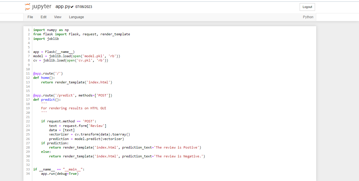
With this code, you can run the Flask application, and it will provide a simple web interface where users can enter a review, and the model will predict the sentiment (positive or negative) of that review.

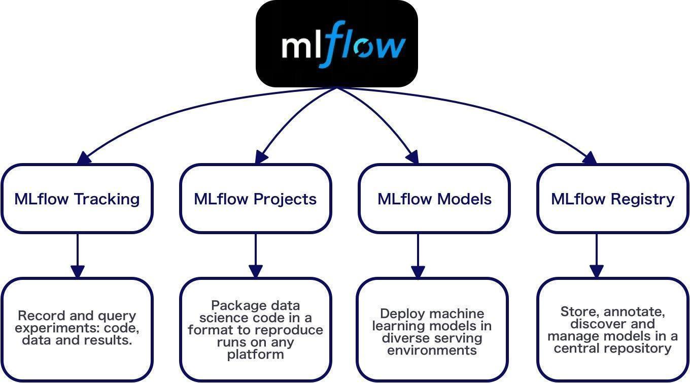
ML FLOW:

MLflow is an open-source platform for managing the end-to-end machine learning lifecycle. It allows you to track experiments, package code, and manage models, making it easier to reproduce, share, and deploy machine learning projects. While MLflow is not specifically designed for text classification, you can use it in a text classification project to keep track of experiments, track metrics, log model artifacts, and more.

Tracking Experiments:

MLflow allows you to track different experiments, including different models, preprocessing techniques, or hyperparameter settings. By using MLflow's tracking functionality, you can log metrics, parameters, and artifacts associated with each experiment. This helps you compare different models and configurations easily.

• What is Mlflow?

MLflow is an open-source platform designed to manage the end-to-end machine learning (ML) lifecycle. It provides a set of tools and components that help data scientists and engineers track, reproduce, deploy, and manage machine learning models effectively. 

• Advanced Mlflow features and integrations

MLflow offers several advanced features and integrations that can enhance your machine learning workflow. Here are some of the notable ones:

1.MLflow Projects: MLflow Projects allow you to package your code and dependencies in a reproducible manner. It provides a standard format for organizing and running your machine learning code, making it easier to reproduce experiments across different environments. MLflow Projects can be run locally, on a remote server, or in a distributed computing environment.

2.MLflow Models: MLflow Models provide a framework-agnostic way to package and share trained machine learning models. MLflow Models also support model versioning, enabling easy management and tracking of model revisions.

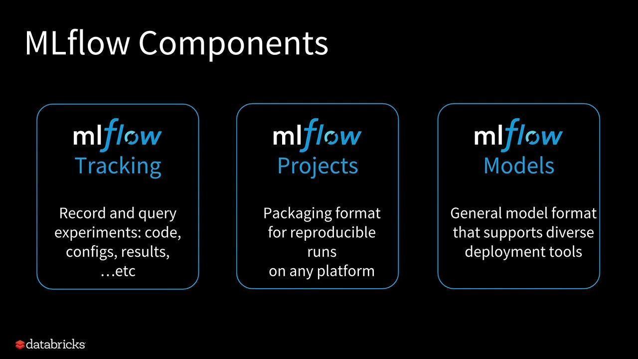
3.MLflow Model Registry: The Model Registry is a central repository for managing and versioning machine learning models. It allows you to register models, track different versions, apply stage transitions (e.g., from "Staging" to "Production"), and control access and permissions. 

4.MLflow Model Serving: MLflow supports model serving through integrations with various serving frameworks and technologies. For example, you can use the MLflow Python REST API to deploy models in cloud platforms. MLflow also provides a built-in model server called MLflow Model Server, which simplifies the process of serving models locally or in production.

5.MLflow Tracking UI and REST API: MLflow provides a user-friendly web-based UI for visualizing and exploring experiment runs, metrics, parameters, and artifacts. You can easily navigate through experiments, compare runs, and access detailed information about each run.

Using ML flow end-to-end to train a linear regression model:

Uses a dataset to predict the quality of wine based on quantitative features like the wine’s “fixed acidity”, “pH”, “residual sugar”, and so on. The dataset is from UCI’s machine learning repository.

At the core, MLflow Projects are just a convention for organizing and describing your code to let other data scientists (or automated tools) run it. Each project is simply a directory of files, or a Git repository, containing your code. MLflow can run some projects based on a convention for placing files in this directory (for example, a conda.

The need:

you’ll need to:

• Install MLflow and scikit-learn. There are two options for installing these dependencies:
  1. Install MLflow with extra dependencies, including scikit-learn (via pip install mlflow[extras])
  2. Install MLflow (via pip install mlflow) and install scikit-learn separately (via pip install scikit-learn)
• Install conda
• Clone (download) the MLflow repository via git clone https://github.com/mlflow/mlflow
• cd into the examples directory within your clone of MLflow - we’ll use this working directory for running the tutorial. We avoid running directly from our clone of MLflow as doing so would cause the tutorial to use MLflow from source, rather than your PyPI installation of MLflow.

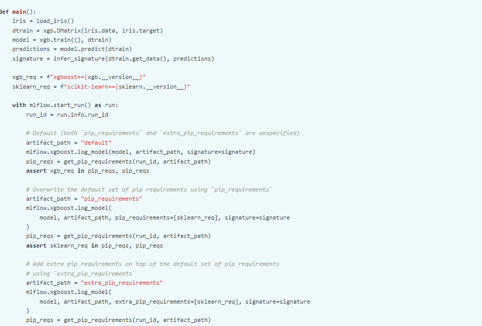
TRAINING THE MODEL:

First, train a linear regression model that takes two hyperparameters: alpha and l1_ratio.

This example uses the familiar pandas, numpy, and sklearn APIs to create a simple machine learning model. The ML flow tracking APIs log information about each training run, like the hyperparameters alpha and l1_ratio, used to train the model and metrics, like the root mean square error, used to evaluate the model. The example also serializes the model in a format that MLflow knows how to deploy.

You can run the example with default hyperparameters as follows:

python sklearn_elasticnet_wine/train.py

Try out some other values for alpha and l1_ratio by passing them as arguments to train.py:

python sklearn_elasticnet_wine/train.py <alpha> <l1_ratio>

Each time you run the example, MLflow logs information about your experiment runs in the directory mlruns.

COMPARING THE MODELS:

Next, use the MLflow UI to compare the models that you have produced. In the same current working directory as the one that contains the mlruns run:

mlflow ui

and view it at http://localhost:5000.

On this page, you can see a list of experiment runs with metrics you can use to compare the models.

You can use the search feature to quickly filter out many models. For example, the query metrics.rmse < 0.8 returns all the models with root mean squared error less than 0.8. For more complex manipulations, you can download this table as a CSV and use your favorite data munging software to analyze it.

PACKAGING TRAINING CODE IN A CONDA ENVIRONMENT:

Now that you have your training code, you can package it so that other data scientists can easily reuse the model, or so that you can run the training remotely.

entry_points:

  main:

    parameters:

      alpha: {type: float, default: 0.5}

      l1_ratio: {type: float, default: 0.1}

    command: "python train.py {alpha} {l1_ratio}"

sklearn_elasticnet_wine/conda.yaml file lists the dependencies:

dependencies:

  - python=3.8

  - pip

  - pip:

      - scikit-learn==1.2.0

      - mlflow>=1.0

      - pandas

To run this project, invoke mlflow run sklearn_elasticnet_wine -P alpha=0.42. After running this command, MLflow runs your training code in a new Conda environment with the dependencies specified in conda

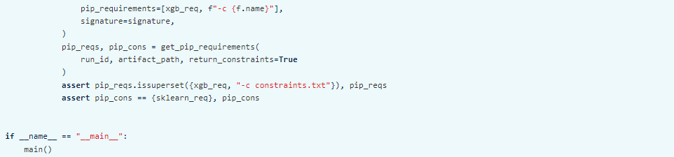
Specifying pip requirements using pip_requirements and extra_pip_requiements:

SERVING THE MODEL:

Now that you have packaged your model using the MLproject convention and have identified the best model, it is time to deploy the model using some ml flow models. An MLflow Model is a standard format for packaging machine learning models that can be used in a variety of downstream tools — for example, real-time serving through a REST API or batch inference on Apache Spark.

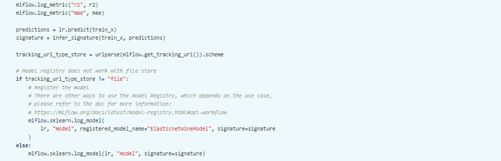
In the example training code, after training the linear regression model, a function in MLflow saved the model as an artifact within the run.

mlflow.sklearn.log_model(lr, "model")

To view this artifact, you can use the UI again

At the bottom, you can see that the call to mlflow.sklearn.log_model produced two files in /Users/mlflow/mlflow-prototype/mlruns/0/7c1a0d5c42844dcdb8f5191146925174/artifacts/model. The first file, MLmodel, is a metadata file that tells MLflow how to load the model. The second file, model.pkl, is a serialized version of the linear regression model that you trained.

In this example, you can use this MLmodel format with MLflow to deploy a local REST server that can serve predictions.

To deploy the server, run (replace the path with your model’s actual path):mlflow models serve Once you have deployed the server, you can pass it some sample data and see the predictions.

DEPLOY THE MODEL:

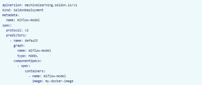
After training and testing our model, we are now ready to deploy it to production, To build a Docker image containing our model, we can use the  subcommand, alongside the --enable-mlserver flag. For example, to build a image named my-docker-image, we could do:

Code:

mlflow models build-docker \

  -m /Users/mlflow/mlflow-prototype/mlruns/0/7c1a0d5c42844dcdb8f5191146925174/artifacts/model \

  -n my-docker-image \

  --enable-mlserver

Once we have our image built, the next step will be to deploy it to our cluster. One way to do this is by applying the respective Kubernetes manifests through the kubectl CLI:

kubectl apply -f my-manifest.yaml

CONCLUSION:

In conclusion, text classification is a vital component of NLP and has numerous applications across various industries. Choosing appropriate feature representation, model selection, data quality, and evaluation metrics are critical for building effective text classifiers. The field of text classification continues to evolve, and leveraging the latest advancements can lead to better performing models for various text-related tasks.

Do Checkout:

1.The link  to our product named AIEnsured offers explainability and many more techniques.

2.To know more about explainability and AI-related articles  please visit this link.

References:

1.https://towardsdatascience.com/keeping-up-with-the-berts-5b7beb92766

2.https://towardsdatascience.com/word2vec-explained-49c52b4ccb71

3.https://towardsdatascience.com/text-classification-using-naive-bayes-theory-a-working-example-2ef4b7eb7d5a

4.https://mlflow.org/

5.https://cloud.google.com/ai-platform/training/docs/algorithms/bert-star

Written by - Poluparthi Supriya

.