CNN and LSTM Overview

A Convolutional Neural Network (CNN) is a type of Deep Learning neural network architecture commonly used in Computer Vision. Computer vision is a field of Artificial Intelligence that enables a computer to understand and interpret the image or visual data. 

 In a regular Neural Network there are three types of layers:

1. Input Layers: It’s the layer in which we give input to our model. The number of neurons in this layer is equal to the total number of features in our data (number of pixels in the case of an image).
2. Hidden Layer: The input from the Input layer is then fed into the hidden layer. There can be many hidden layers depending upon our model and data size. Each hidden layer can have different numbers of neurons which are generally greater than the number of features. The output from each layer is computed by matrix multiplication of output of the previous layer with learnable weights of that layer and then by the addition of learnable biases followed by activation function which makes the network nonlinear.
3. Output Layer: The output from the hidden layer is then fed into a logistic function like sigmoid or softmax which converts the output of each class into the probability score of each class.

Convolution Neural Network

Convolutional Neural Network (CNN) is the extended version of artificial neural 

networks (ANN) which is predominantly used to extract the feature from the grid-like matrix dataset. For example visual datasets like images or videos where data patterns play an extensive role.

CNN architecture

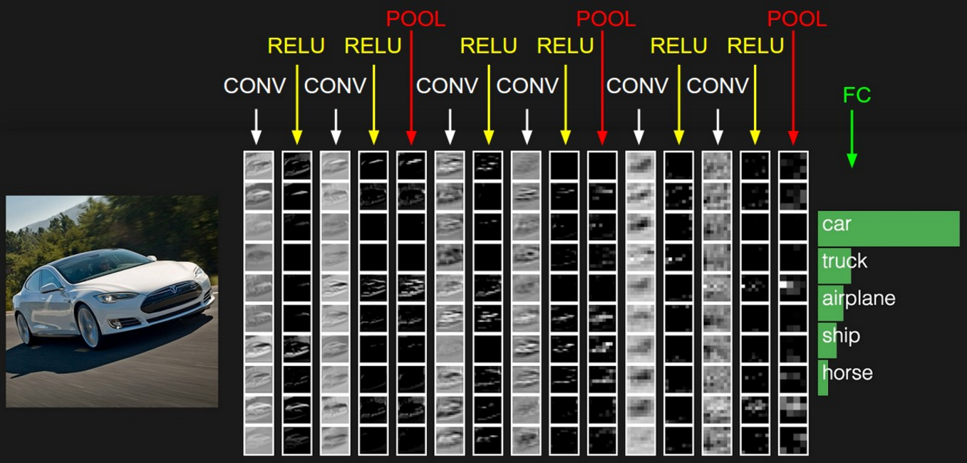
Convolutional Neural Network consists of multiple layers like the input layer, Convolutional layer, Pooling layer, and fully connected layers. 

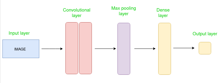
The Convolutional layer applies filters to the input image to extract features, the Pooling layer downsamples the image to reduce computation, and the fully connected layer makes the final prediction. The network learns the optimal filters through backpropagation and gradient descent.

How Convolutional Layers works

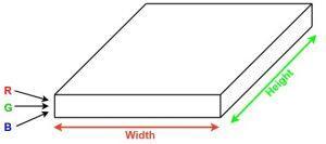
Convolutional Neural Networks or covers are neural networks that share their parameters. Imagine you have an image. It can be represented as a cuboid having its length, width (dimension of the image), and height (i.e the channel as images generally have red, green, and blue channels). 

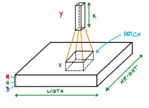
Now imagine taking a small patch of this image and running a small neural network, called a filter or kernel on it, with say, K outputs and representing them vertically. Now slide that neural network across the whole image, as a result, we will get another image with different widths, heights, and depths. Instead of just R, G, and B channels now we have more channels but lesser width and height. This operation is called Convolution. If the patch size is the same as that of the image it will be a regular neural network. Because of this small patch, we have fewer weights. 

Now let’s talk about a bit of mathematics that is involved in the whole convolution process. 

• Convolution layers consist of a set of learnable filters (or kernels) having small widths and heights and the same depth as that of input volume (3 if the input layer is image input).
• For example, if we have to run convolution on an image with dimensions 34x34x3. The possible size of filters can be xx3, where ‘a’ can be anything like 3, 5, or 7 but smaller as compared to the image dimension.
• During the forward pass, we slide each filter across the whole input volume step by step where each step is called stride (which can have a value of 2, 3, or even 4 for high-dimensional images) and compute the dot product between the kernel weights and patch from input volume.
• As we slide our filters we’ll get a 2-D output for each filter and we’ll stack them together as a result, we’ll get output volume having a depth equal to the number of filters. The network will learn all the filters.

Layers used to build ConvNets

A complete Convolution Neural Networks architecture is also known as covnets. A covnets is a sequence of layers, and every layer transforms one volume to another through a differentiable function. Types of layers: datasetsLet’s take an example by running a covnets on of image of dimension 32 x 32 x 3. 

• Input Layers: It’s the layer in which we give input to our model. In CNN, Generally, the input will be an image or a sequence of images. This layer holds the raw input of the image with width 32, height 32, and depth 3.
• Convolutional Layers: This is the layer, which is used to extract the feature from the input dataset. It applies a set of learnable filters known as the kernels to the input images. The filters/kernels are smaller matrices usually 2×2, 3×3, or 5×5 shape. it slides over the input image data and computes the dot product between kernel weight and the corresponding input image patch. The output of this layer is referred ad feature maps. Suppose we use a total of 12 filters for this layer we’ll get an output volume of dimension 32 x 32 x 12.
• Activation Layer: By adding an activation function to the output of the preceding layer, activation layers add nonlinearity to the network. it will apply an element-wise activation function to the output of the convolution layer. Some common activation functions are RELU: max(0, x),  Tanh, Leaky RELU, etc. The volume remains unchanged hence output volume will have dimensions 32 x 32 x 12.
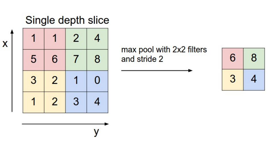
• Pooling layer: This layer is periodically inserted in the covnets and its main function is to reduce the size of volume which makes the computation fast reduces memory and also prevents overfitting. Two common types of pooling layers are max pooling and average pooling. If we use a max pool with 2 x 2 filters and stride 2, the resultant volume will be of dimension 16x16x12. 

• Flattening: The resulting feature maps are flattened into a one-dimensional vector after the convolution and pooling layers so they can be passed into a completely linked layer for categorization or regression.
• Fully Connected Layers: It takes the input from the previous layer and computes the final classification or regression task.

• Output Layer: The output from the fully connected layers is then fed into a logistic function for classification tasks like sigmoid or softmax which converts the output of each class into the probability score of each class.

Advantages of Convolutional Neural Networks (CNNs):

1. Good at detecting patterns and features in images, videos, and audio signals.
2. Robust to translation, rotation, and scaling invariance.
3. End-to-end training, no need for manual feature extraction.
4. Can handle large amounts of data and achieve high accuracy.

Disadvantages of Convolutional Neural Networks (CNNs):

1. Computationally expensive to train and require a lot of memory.
2. Can be prone to overfitting if not enough data or proper regularization is used.
3. Requires large amounts of labeled data.
4. Interpretability is limited, it’s hard to understand what the network has learned.

CNN (Convolutional Neural Network or ConvNet) is a type of feed-forward artificial network where the connectivity pattern between its neurons is inspired by the organization of the animal visual cortex. The visual cortex has a small region of cells that are sensitive to specific regions of the visual field.

CNN is not supervised or unsupervised, it's just a neural network that, for example, can extract features from images by dividing it, pooling and stacking small areas of the image.

A convolutional neural network (CNN or convnet) is a subset of machine learning.

LSTM(LONG SHORT TERM MEMORY)

To solve the problem of Vanishing and Exploding Gradients in a Deep Recurrent Neural Network, many variations were developed. One of the most famous of them is the Long Short Term Memory Network(LSTM). In concept, an LSTM recurrent unit tries to “remember” all the past knowledge that the network is seen so far and to “forget” irrelevant data. This is done by introducing different activation function layers called “gates” for different purposes. Each LSTM recurrent unit also maintains a vector called the Internal Cell State which conceptually describes the information that was chosen to be retained by the previous LSTM recurrent unit.

LSTM networks are the most commonly used variation of Recurrent Neural Networks (RNNs). The critical component of the LSTM is the memory cell and the gates (including the forget gate but also the input gate), inner contents of the memory cell are modulated by the input gates and forget gates. Assuming that both of the segue he are closed, the contents of the memory cell will remain unmodified between one time-step and the next gradients gating structure allows information to be retained across many time-steps, and consequently also allows group that to flow across many time-steps. This allows the LSTM model to overcome the vanishing gradient properly occurs with most Recurrent Neural Network models.

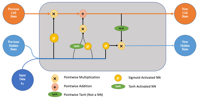
 A Long Short Term Memory Network consists of four different gates for different purposes as described below:- 

1. Forget Gate(f): At forget gate the input is combined with the previous output to generate a fraction between 0 and 1, that determines how much of the previous state need to be preserved (or in other words, how much of the state should be forgotten). This output is then multiplied with the previous state. Note: An activation output of 1.0 means “remember everything” and activation output of 0.0 means “forget everything.” From a different perspective, a better name for the forget gate might be the “remember gate”
2. Input Gate(i): Input gate operates on the same signals as the forget gate, but here the objective is to decide which new information is going to enter the state of LSTM. The output of the input gate (again a fraction between 0 and 1) is multiplied with the output of tan h block that produces the new values that must be added to previous state. This gated vector is then added to previous state to generate current state
3. Input Modulation Gate(g): It is often considered as a sub-part of the input gate and much literature on LSTM’s does not even mention it and assume it is inside the Input gate. It is used to modulate the information that the Input gate will write onto the Internal State Cell by adding non-linearity to the information and making the information Zero-mean. This is done to reduce the learning time as Zero-mean input has faster convergence. Although this gate’s actions are less important than the others and are often treated as a finesse-providing concept, it is good practice to include this gate in the structure of the LSTM unit.
4. Output Gate(o): At output gate, the input and previous state are gated as before to generate another scaling fraction that is combined with the output of tanh block that brings the current state. 

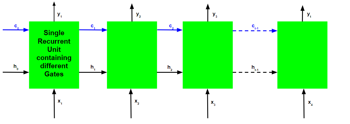
The basic workflow of a Long Short Term Memory Network is similar to the workflow of a Recurrent Neural Network with the only difference being that the Internal Cell State is also passed forward along with the Hidden State. 

Working of an LSTM recurrent unit:  

1. Take input the current input, the previous hidden state, and the previous internal cell state.
2. Calculate the values of the four different gates by following the below steps:-
   • For each gate, calculate the parameterized vectors for the current input and the previous hidden state by element-wise multiplication with the concerned vector with the respective weights for each gate.
   • Apply the respective activation function for each gate element-wise on the parameterized vectors. Below given is the list of the gates with the activation function to be applied for the gate.
3. Calculate the current internal cell state by first calculating the element-wise multiplication vector of the input gate and the input modulation gate, then calculate the element-wise multiplication vector of the forget gate and the previous internal cell state and then add the two vectors. 
4. Calculate the current hidden state by first taking the element-wise hyperbolic tangent of the current internal cell state vector and then performing element-wise multiplication with the output gate.

The above-stated working is illustrated as below:-  

Note that the blue circles denote element-wise multiplication. The weight matrix W contains different weights for the current input vector and the previous hidden state for each gate. 

Just like Recurrent Neural Networks, an LSTM network also generates an output at each time step and this output is used to train the network using gradient descent. 

The only main difference between the Back-Propagation algorithms of Recurrent Neural Networks and Long Short Term Memory Networks is related to the mathematics of the algorithm. 

This post explains long short-term memory (LSTM) networks. I find that the best way to learn a topic is to read many different explanations and so I will link some other resources I found particularly helpful, at the end of this article. I would highly encourage you to check them out for varying perspectives and explanations of LSTMs!

References: