Accumulated Local Effects (ALE) Plot in Audio Classification

Model explainability refers to the concept of being able to understand the machine learning model. Being able to interpret a model increases trust in AI. There are two ways to interpret a model i.e. Global vs Local Interpretation.
Global interpretation helps us in understanding how a model makes decisions for the overall structure, whereas Local interpretation helps in understanding how a model makes decisions for a single instance.
In the previous article, we have seen how to build an Audio Classifier and used SHAP on that. Here in this blog, we will talk about the Accumulated Local Effects (ALE) plot, which is a kind of Global Interpretation.
Why Accumulated Local Effects (ALE)?
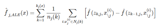
Accumulated local effects(ALE) plots to highlight the effects that specific features have on the predictions of a machine learning model by partially isolating the effects of other features. The resulting ALE explanation is centered around the mean effect of the feature, such that the main feature effect is compared relative to the average prediction of the data.
To estimate local effects, we divide the feature into many intervals and compute the differences in the predictions. This procedure approximates the derivatives and also works for models without derivatives.
Advantages of using ALE plots :
- ALE plots are unbiased, which means they still work when features are correlated.
- The interpretation of ALE plots is clear: Conditional on a given value, the relative effect of changing the feature on the prediction can be read from the ALE plot.
- ALE plots are centered at zero. This makes their interpretation nice because the value at each point of the ALE curve is the difference from the mean prediction. The 2D ALE plot only shows the interaction: If two features do not interact, the plot shows nothing.
What difference does ALE bring from SHAP?
ALE helps in interpreting the feature importance based on their values at the whole data level and presents in form of plots, whereas SHAP tells us how the feature is important for a particular class label based on shapely values.
So, both the techniques have their own importance. Now, let's dive into the ALE.
Once we have the Audio classifier (refer to the previous article) with us, we will install ALE using the pip command and after converting the data from 2D to a 1D array by averaging the rows, we will use ALE's explain function to get the ALE plots.
ale = ALE(pred_fn_shap_ale, target_names=class_names, feature_names = feat)
exp = ale.explain(X, features=top5_feat)
The following figures show the Accumulated Local Effects (ALE) plots for the audio classification model trained on the music dataset for the respective features.
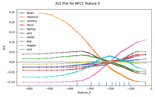
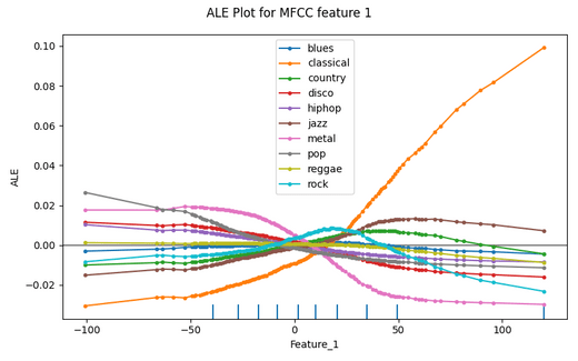
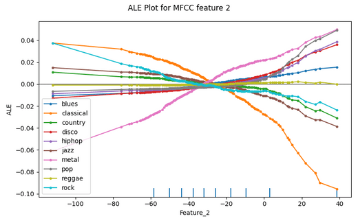
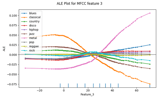
So, in the plots above we can see how ALE shows the importance of feature at the class level by showing in which interval the feature is important for the respective class.
For example, let's consider Feature_3 and look for the classical class label (orange color). we can clearly see that, when the feature's values were below 20, it was having a high influence on prediction for classical class, whereas when the values were above 20, it was having less influence for the same, similarly we can see for other classes and other features from the plots above.
In this way, Accumulated Local Effects (ALE) helps in looking at the effects that specific features have on the predictions of a machine learning model.
References :
- https://blog.testaing.com/shap-feature-importance-in-audio-classification/
- https://christophm.github.io/interpretable-ml-book/ale.html
- https://docs.oracle.com/en-us/iaas/tools/ads-sdk/latest/user_guide/mlx/accumulated_local_effects.html