Unveiling The Essence of Topic Classification Using BERT

In this article, let's explore BERT which is the pre-trained model from Hugging Face Transformers, before diving deeper into it. It was introduced by Google back in 2018. BERT (Bidirectional Encoder Representations from Transformers) is a pre-trained language model that has revolutionized the way we understand and process text.
What makes BERT special is its ability to grasp the contextual meaning of words and sentences. Through extensive training on large amounts of text data, BERT has learned to understand the relationships between words, unlocking a new level of comprehension.
With BERT as your guide, you can navigate through complex text and extract valuable insights. From sentiment analysis to document classification, BERT empowers you to tackle a wide range of natural language processing tasks with confidence and accuracy.
Join us as we delve into the world of BERT and explore its ability in topic classification.
DATASET :
We are going to use a BBC news classification dataset for text classification task. It consists of news articles from the BBC website, spanning five different categories: business, entertainment, politics, sports and technology.

This dataset provides a diverse range of text samples, making it suitable for training and evaluating models for multi-class text classification. Each text is labelled with one of the five categories, allowing for supervised learning approaches.
You can download the dataset via: https://storage.googleapis.com/dataset-uploader/bbc/bbc-text.csv
DATA PREPROCESSING :
Data preprocessing means the essential steps taken to transform raw data into a format that is suitable for analysis or modelling. It involves cleaning and transforming the data to ensure its quality. This involves removing irrelevant data, handling missing values, normalizing numerical features, encoding categorical features and performing text preprocessing tasks like tokenization and removing stop words.
Let’s get started:
We are using sample function to shuffle the data to ensure that similar categories are not grouped together. Here, rename function is being used to change the name of the columns.
datapath = f'/content/archive.zip'
df = pd.read_csv(datapath)
df = df.sample(frac=1, random_state=1).reset_index(drop=True)
df = df.rename(columns={'text':'description'})
df.head()
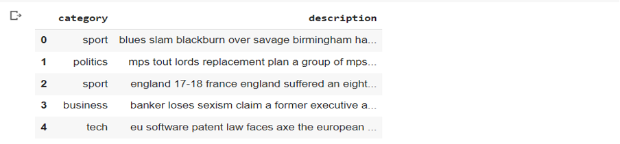
Before preprocessing, let’s get a glimpse of the text.
- Lower casing:
Lower casing is performed in text preprocessing to normalize the text by converting all letters to lowercase. This ensures that words with different cases are treated as the same word, reducing the vocabulary size and avoiding duplication of information in the model, as "apple" and "Apple" would be considered the same word.
# Convert to lower case
df['description'] = df['description'].str.lower()
2. Removing HTML Tags:
This step is necessary in text preprocessing to extract meaningful information from web documents. HTML tags, such as <div>, <p>, <a>, or <b>, carry no meaningful information for many text analysis tasks and can introduce noise or irrelevant features. Removing these help to solely focus on the text.
# Remove html tags
import re
def remove_html_tegs(text):
pattern = re.compile('<.*?>')
return pattern.sub(r'',text)
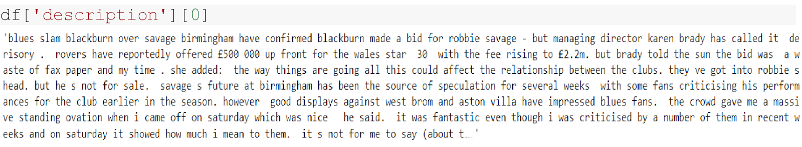
df['description'] = df['description'].apply(remove_html_tegs)
df['description'][0]
3. Remove Punctuation:
Punctuation marks like full stops, commas, question marks, and exclamation points do not typically carry significant meaning on their own in many text analysis tasks. So, often we remove them.
# Remove punctuation
import string
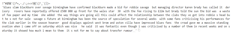
print(string.punctuation)
exclude = string.punctuation
def remove_punc(text):
return text.translate(str.maketrans('','',exclude))
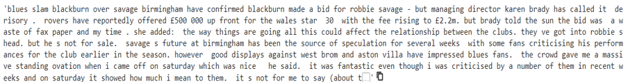
df['description'] = df['description'].apply(remove_punc)
df['description'][0]
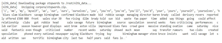
4. Remove Stopwords:
Stopwords such as common words like "and," "the," and "is," are required only for sentence formation, so removing them helps focus on more meaningful and informative words in text analysis.
# Removing stopwords
import nltk
nltk.download('stopwords')
from nltk.corpus import stopwords
print(list(stopwords.words('english')))
def remove_stopwords(text):
    new_text = []
    for word in text.split():
        if word in stopwords.words('english'):
            new_text.append('')
        else:
            new_text.append(word)
    x = new_text[:]
    new_text.clear()
    return ' '.join(x)
df['description'] = df['description'].apply(remove_stopwords)
df['description'][0]
5. Replace missing values and visualize data:
First, we will check if the rows and columns contain any missing values.

Since, there are no missing values we need not do anything. If there are any missing values in the dataset you can replace it using fillna() function.
print(df.category.value_counts())
df.groupby(['category']).size().plot.bar()

TOKENIZER :
BERT base cased tokenizer has the power to understand and break down complex sentences into smaller, meaningful pieces called tokens. Let’s say you have the sentence: "The quick brown fox jumps over the lazy dog." After tokenization, it would be split into individual tokens: ["The", "quick", "brown", "fox", "jumps", "over", "the", "lazy", "dog", "."]. These tokens capture essential details while maintaining the integrity of the original words. Each token represents a meaningful unit of text, making it easier for the BERT model to understand and process the input effectively. To learn more about the tokenizers, refer to this link.
# Bert Tokenizer - splits a sentence into tokens and adds special characters at the start and end of the sentence
tokenizer = BertTokenizer.from_pretrained('bert-base-cased')
# Mapping the classes
classes = {'business': 0, 'entertainment': 1, 'sport': 2, 'tech': 3, 'politics': 4}
Now, we will create a dataset class to get the data in batches for training, validation and testing.
# Create batches using the dataset
class Dataset_(Dataset):
    def __init__(self, df):

        self.classes = [classes[label] for label in df['category']]
        self.descriptions = [tokenizer(description, padding='max_length', max_length = 512, truncation=True, return_tensors="pt")
                                  for description in df['description']]

    def __len__(self):
        # Get the number of classes
        return len(self.classes)

    def __getitem__(self, idx):
        return self.descriptions[idx], self.classes[idx]
CREATING MODEL :
Now, we will create a model by fine-tuning the BERT model to perform the text classification task into five different categories. We are going to use bert-base-cased model as our dataset is in English language.
The BERT model returns two outputs: one the word embeddings vector and the other is the previous output from the decoder. It is then passed through a linear layer to perform the text classification into 5 categories.
# Bert Classifier model
class BertClassifier(nn.Module):
    def __init__(self, dropout=0.6):

        super(BertClassifier, self).__init__()

        self.bert = BertModel.from_pretrained('bert-base-cased')
        self.dropout = nn.Dropout(dropout)
        self.linear = nn.Linear(768, 5)

    def forward(self, input_id, mask):

        _, output = self.bert(input_ids= input_id, attention_mask=mask,return_dict=False)
        output = self.dropout(output)
        output = F.relu(self.linear(output))

    return output
TRAINING AND EVALUATING MODEL :
The next step after creating the model is to train and evaluate our model. Firstly, we will split the dataset into train, validation and test datasets using the split function.
df_train, df_val, df_test = np.split(df.sample(frac=1, random_state=42), [int(.7*len(df)), int(.9*len(df))])
After this, we use train and evaluate functions to test our model accuracy.
Epochs = 3
model = BertClassifier()
lr = 1e-6
batch_size = 2

train(model, df_train, df_val, lr, Epochs, batch_size)
After training the model for 3 epochs, these are the results that I have obtained:

By training the model for 3 epochs, we are obtaining a test accuracy of around 94% which is a pretty good result. The training accuracy may vary depending on the randomness of the data and number of epochs.
CLASSIFICATION REPORT :
Classification report is used to evaluate the performance of your model. It is used to show precision, recall, F1 score and support of the trained classification model.
Let’s breakdown and understand the terms in a classification report:
- Precision: It tells us how many things we predicted as positive actually belong to the positive class. If precision is high, it means we are making fewer mistakes.
- Recall: Recall is like being thorough. It tells us how many of the actual positive things we managed to find. If recall is high, it means we are not missing many positive things in our predictions.
- F1 score: It is like a balanced measure between precision and recall. It combines both the aspects to give an overall score that tells how well the model is performing.
- Support: It is the number of samples for each class in the dataset. It tells us how many instances of each category to predict on.
- Accuracy: It tells us how many predictions we got right out of all the predictions made.
Here, we can see the classification report for our model:

CONFUSION MATRIX :
A confusion matrix is a powerful tool that provides valuable insights into the performance of our model, specifically in classification tasks. By visually representing the model's predictions and their agreement with the true labels, the confusion matrix allows us to evaluate the accuracy and identify any patterns of misclassifications. Let's explore the code and understand the significance of the confusion matrix in evaluating our machine learning model. The evaluation code can be updated to include the confusion matrix for our model as follows :
def evaluate(model, test_data, batch_size):
test = Dataset_(test_data)
test_dataloader = DataLoader(test, batch_size=batch_size)

use_cuda = torch.cuda.is_available()
device = torch.device("cuda" if use_cuda else "cpu")

if use_cuda:
    model = model.cuda()

total_acc_test = 0
y_true = []
y_pred = []

with torch.no_grad():
    for test_input, test_label in tqdm(test_dataloader):
        test_label = test_label.to(device)
        mask = test_input['attention_mask'].to(device)
        input_id = test_input['input_ids'].squeeze(1).to(device)

        output = model(input_id, mask)

        y_true.extend(test_label.cpu().numpy())
        y_pred.extend(output.argmax(dim=1).cpu().numpy())

        acc = (output.argmax(dim=1) == test_label).sum().item()
        total_acc_test += acc

print(f'Test Accuracy: {total_acc_test / len(test_data): .3f}')

# Compute and display the confusion matrix
labels = ['business', 'entertainment', 'sport', 'tech', 'politics']
cm = confusion_matrix(y_true, y_pred)
plot_confusion_matrix(cm, labels)

def plot_confusion_matrix(cm, labels):
plt.figure(figsize=(8, 6))
sns.heatmap(cm, annot=True, fmt='d', cmap='Blues', xticklabels=labels, yticklabels=labels)
plt.xlabel('Predicted Labels')
plt.ylabel('True Labels')
plt.title('Confusion Matrix')
plt.show()

evaluate(model, df_test, batch_size)
The output of the above code is shown in the image below:
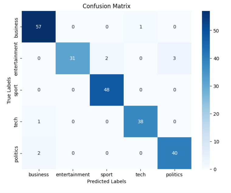
The row sum gives the number of samples of each class in the test dataset. By identifying the patterns between true labels and predicted labels, we can evaluate the accuracy of our model for each class.
IMPLEMENTATION OF MLFLOW :
MLflow is an open-source platform that helps manage and track machine learning experiments. It allows beginners to easily record and compare models, track parameters and metrics, and reproduce results. MLflow provides a simple way to organize and share ML projects, making it easier to collaborate and iterate on models.
Below is the code snippet that displays the integration of MLflow into the model:
import mlflow
import mlflow.pytorch

params = {"epochs": 2, "learning_rate": 1e-6, "batch_size": 2}
metrics = {"final_train_loss": train_losses[-1], "final_train_accuracy": train_accuracies[-1], 	   "final_val_loss": val_losses[-1], "final_val_accuracy": val_accuracies[-1],
       "final_test_accuracy": test_accuracies[-1]}
experiment_name = "Bert classifier"
model_artifact_path = "model"
plot_artifact_path = "metrics_plot.png"
with mlflow.start_run(run_name="bert", nested=True) as run:
mlflow.set_experiment(experiment_name)

for key, value in params.items():
    mlflow.log_param(key, value)

model = BertClassifier()
model, train_losses, train_accuracies, val_losses, val_accuracies = train(model, df_train,  df_val, params["learning_rate"], params["epochs"], params["batch_size"])

model, test_accuracies = evaluate(model, df_test, params["batch_size"])

for key, value in metrics.items():
    mlflow.log_metric(key, value)

# Log training and validation accuracy curves
plt.figure(figsize=(10, 6))
plt.plot(range(1, params["epochs"] + 1),train_accuracies, label="Training Accuracy")
plt.plot(range(1, params["epochs"] + 1),val_accuracies, label="Validation Accuracy")
plt.xlabel("Epochs")
plt.ylabel("Accuracy")
plt.title("Training and Validation Accuracy Curves")
plt.legend()
plt.savefig("accuracy_curves.png")
mlflow.log_artifact("accuracy_curves.png")
 # The above code can be used to Log training and validation loss curves, test accuracy curve
mlflow.pytorch.log_model(model, model_artifact_path)

mlflow.end_run()
In the above code snippet, MLflow is used to track parameters, metrics, plot loss and accuracy curves. The ‘mlflow.start_run()’ function starts a new MLflow run, and ‘mlflow.log_param()’ and ‘mlflow.log_metric()’ are used to log the parameters and metrics, respectively. The trained model is saved using ‘mlflow.pytorch.log_model()’. Finally, the model results are displayed in the MLflow user interface where you can visualize and track the experiment results.
DEPLOYMENT USING FLASK :
Flask is a lightweight web framework for building web applications in Python. It helps beginners create simple web applications by handling HTTP requests, routing URLs, and rendering the HTML templates. Flask is flexible, easy to learn, and widely used in the Python community.
Below is the code snippet showcasing a Flask application that incorporates HTML files to serve our model:
from flask import Flask, request, jsonify, render_template
import torch
import numpy as np
import os
from transformers import BertTokenizer, BertModel
from torch import nn
import torch.nn.functional as F

app = Flask(__name__)

tokenizer = BertTokenizer.from_pretrained('bert-base-cased')
classes = {'Business': 0, 'Entertainment': 1, 'Sport': 2, 'Tech': 3, 'Politics': 4}
# Include the code of the Bert Classifier model over here
model = BertClassifier()
model.load_state_dict(torch.load('model.pt'))
model.eval()

@app.route('/', methods=['GET', 'POST'])
def index():
    if request.method == 'POST':
    text = request.form['text']
    inputs = tokenizer(text, padding='max_length', max_length=512, truncation=True, return_tensors="pt")
    input_id = inputs['input_ids']
    mask = inputs['attention_mask']
    with torch.no_grad():
        outputs = model(input_id, mask)
        probabilities = torch.nn.functional.softmax(outputs, dim=-1).tolist()[0]
        probabilities = [round(prob, 4) for prob in probabilities]
        predicted_output = np.argmax(probabilities)
        class_name = list(classes.keys())[list(classes.values()).index(predicted_output)]

    return render_template('result.html', probabilities=probabilities, output=class_name)
else:
    return render_template('index.html')

if __name__ == '__main__':
    app.run(debug=True)
This code snippet sets up a Flask web application. The index route renders an index.html template, which typically contains a form for user input. On submitting the form, the index route processes the user's input, performs a prediction using the model, and renders a result.html template to display the prediction. You can also add styling to the HTML files using CSS. Running the Flask app will start the web server, and it can be accessed via your browser to interact with the model. The below image shows an example on how it works :

On submitting the above, the result is shown along with the predicted probability for each class:

LIME EXPLAINABILITY :
LIME (Local Interpretable Model-agnostic Explanations) is a popular method for explaining the predictions of machine learning models. It will help you understand how LIME provides interpretable insights by highlighting the important features contributing to each prediction. Here's a code snippet to showcase LIME's explainability for the model:
!pip install lime
from lime import lime_text
from lime.lime_text import LimeTextExplainer

def predict_fn(texts):
    input_ids = tokenizer.batch_encode_plus(texts, padding='max_length', max_length=512, truncation=True, return_tensors="pt")['input_ids']
    mask = input_ids.ne(tokenizer.pad_token_id)
    input_ids = input_ids.to(device)
    mask = mask.to(device)
    with torch.no_grad():
        output = model(input_ids, mask)
        probabilities = torch.softmax(output, dim=1).cpu().numpy()
    return probabilities

sample_text = df.iloc[5]['description']

explainer = LimeTextExplainer(class_names=list(classes.keys()))

def explain_instance(text):
    explanation = explainer.explain_instance(text, predict_fn, num_features=10, num_samples=200)
    explanation.show_in_notebook(text=text)

explain_instance(sample_text)

To gain a deeper understanding on LIME explainability, make sure to check out this link.
REFERENCES :
- https://towardsdatascience.com/text-classification-with-bert-in-pytorch-887965e5820f
- https://colab.research.google.com/github/abhimishra91/transformers-tutorials/blob/master/transformers_multi_label_classification.ipynb#scrollTo=md9-Q1v6zqmR
- https://huggingface.co/docs/transformers/model_doc/bert
ALSO CHECKOUT :
- Uncover the transformative potential of our AI testing company and take your products to the next level with just one click over here.
- To read more awesome articles on AI and machine learning, check out our Knowledge Hub.
By Soumya G