SHAP Feature Importance in Text Classification

In this blog, we'll be primarily focused on the text classification task of Natural language processing (NLP). We'll be using quality entertainment resources called Rotten Tomatoes and the Tomato meter score online aggregator of movie and TV show reviews from critics, which provide fans with a comprehensive guide to what’s fresh – and what’s Rotten – in theaters and at home. We have created a visualization explaining which words contributed to the predictions.
Why do we need to train the model with important features?
Feature importance allows us to understand the relationship between the input features and the target variable. It also helps you understand what features are irrelevant to the model.
What happens when we train models with irrelevant features?
We all have heard the saying “Garbage in, garbage out”. Similarly when we train a machine learning model with irrelevant features then the model predictions will become irrelevant.
There’s always a case in NLP of feature dimensions being very huge. Which makes explaining feature importance very complicated.
SHAP (SHapley Additive exPlanations) by Lundberg and Lee is a method to explain individual predictions. SHAP is based on the game theoretically optimal Shapley values.
For Tree-based models and ensembles of trees, Tree SHAP can be used and for kernel-based models, we have Kernel SHAP.
Tree SHAP is a fast and exact method to estimate SHAP values under several different possible assumptions about feature dependence.
To compute the importance of each feature in the given text we use a special weighted linear regression called Kernel SHAP. The computed importance values are Shapley values from game theory and also coefficients from a local linear regression.
Why SHAP over LIME?
LIME (Local Interpretable Model-agnostic Explanations) is another popular framework for feature importance analysis.
A long-standing and well-understood economic theory that guarantees the SHAP predictions are fairly distributed among the features whereas LIME does not guarantee this.
SHAP results provide an easy-to-read global interpretation method based on aggregations of Shapley values and a local view of the model predictions, whereas LIME only offers local interpretations.
The idea behind SHAP feature importance is simple: Features with large absolute Shapley values are important.
Since we want global importance, we average the absolute Shapley values per feature across the data. We sort the features by decreasing importance and plot them.
Now will dive into the coding part by getting your hands dirty:
We are importing the packages of pandas, nltk and bs4, vectorizer, classifier, and evaluation metrics
# Importing the packages
import pandas as pd
import nltk
import re
from bs4 import BeautifulSoup
from sklearn.model_selection import train_test_split
from sklearn.feature_extraction.text import CountVectorizer
from sklearn.ensemble import RandomForestClassifier
from sklearn.metrics import classification_report

nltk.download('punkt')
nltk.download('stopwords')
Preprocessing step: we are removing the HTML tags and lowercase the words, punctuations, symbols, and numbers and split them into tokens to remove stop words and return cleaned text.
REPLACE_BY_SPACE_RE = re.compile('[/(){}\[\]\|@,;]')
BAD_SYMBOLS_RE = re.compile('[^0-9a-z #+_]')
STOPWORDS =nltk.corpus.stopwords.words('english')

def clean_text(text):

    text = BeautifulSoup(text, "lxml").text # HTML decoding
    text = text.lower() # lowercase text
    text = REPLACE_BY_SPACE_RE.sub(' ', text) # replace REPLACE_BY_SPACE_RE symbols by space in text
    text = BAD_SYMBOLS_RE.sub('', text) # delete symbols which are in BAD_SYMBOLS_RE from text
    text = ' '.join(word for word in text.split() if word not in STOPWORDS) # delete stop words from text
    return text
Loading the rotten tomatoes dataset using pandas library, cleaning the reviews, and splitting the dataset into training and testing subsets.
fname='/content/rotten_tomatoes.csv'
df = pd.read_csv(fname,encoding='latin-1')
df['cleaned_review'] = df['reviews'].apply(clean_text)
X_train, X_test, y_train, y_test = train_test_split(df["cleaned_review"], df["labels"], test_size=0.2, random_state=123)
To transform a given text into a vector we’ll use count vectorizer word embedding and apply fit transform on train data and transform on the test data. Here, bow means Bag of words.
bow_vectorizer = CountVectorizer(min_df=5, ngram_range=(1,2), stop_words='english')
bow_x_train = bow_vectorizer.fit_transform(X_train)
bow_x_test = bow_vectorizer.transform(X_test)
The output of the bow x train will be in the sparse matrix so, we are converting it to the dense matrix and adding feature names to the count vectorizer data frame.
count_vect_df = pd.DataFrame(bow_x_test.todense(),
columns=bow_vectorizer.get_feature_names_out())
We are building a random forest classifier with 100 trees and model fitting on trained data and prediction on test data.
# Random forest
rf = RandomForestClassifier(n_estimators = 100,criterion = "gini",max_depth=3, min_samples_leaf=5)
rf.fit(bow_x_train, y_train)
pred_rf = rf.predict(bow_x_test)
print(classification_report(y_test, pred_rf))
The classification report considers precision, recall, f1-score as an evaluation metrics:
# Output
                 precision   recall   f1-score  support

           0       0.71      0.47      0.56      1064
           1       0.60      0.81      0.69      1069

    accuracy                           0.64      2133
   macro avg       0.66      0.64      0.63      2133
weighted avg       0.66      0.64      0.63      2133
Now we will install the SHAP using the below command:
!pip install shap
# Output
Collecting SHAP
  Downloading shap-0.40.0-cp37-cp37m-manylinux2010_x86_64.whl (564 kB)
Since we are using a random forest model we will use a tree explainer and plot a summary plot:
import matplotlib.pyplot as plt
plt.style.use('dark_background')
import shap
explainershap = shap.TreeExplainer(rf)
shap_values = shap.TreeExplainer(rf).shap_values(count_vect_df, check_additivity = False)
shap.summary_plot(shap_values, count_vect_df, plot_type="bar",axis_color='#FFFFFF')
The following figure shows the SHAP feature importance for the random forest trained on the count vectorized rotten tomatoes dataset.
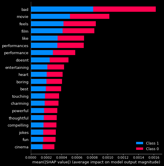
In our bag of words model, SHAP will treat each word in our word vocabulary as an individual feature. We can then map the attribution values to the indices in our vocabulary to see the words that contributed most (and least) to our model’s predictions of whether rotten tomatoes movie reviews 1 for good and 0 for rotten.
One such magical product that offers Model Explainability is AIEnsured by TestAIng.
References:
- Christoph Molnar, “Interpretable machine learning. A Guide for Making Black Box Models Explainable”, 2019.
- Rotten tomatoes Dataset source link.
- https://shap.readthedocs.io/en/latest/example_notebooks/api_examples/plots/text.html
Other articles you can look for:
- https://blog.testaing.com/sklearn-feature-importance-in-text-classification/
- https://blog.testaing.com/lime-technique-for-text-classification/
- https://blog.testaing.com/shap-feature-importance/
- https://blog.testaing.com/poka-yoking-your-ml-model/
By Shiva Kumar